Risk assessment#
A workflow from the CLIMAAX Handbook and MULTI_infrastructure GitHub repository.
See our how to use risk workflows page for information on how to run this notebook.
In this notebook, the calculation of risk associated with the variable under examination will be shown. Pandas dataframes will be presented which, in the example, show nine airports - the operator will need to modify the list of airports by adding/modifying names. The same concept applies to exposure and vulnerability indicators - indicators will be presented that can be expanded or modified by the user. The only mandatory thing is that the framework was conceptualized for at least two airports
Preparation work#
Import libraries#
import os

import matplotlib.pyplot as plt
import numpy as np
import pandas as pd
import scipy.spatial
import xarray as xr
import contextily

import plotly.express as px
Area of interest#
Specify the same name as in the the hazard assessment to continue with the results of these notebooks.
region_name = 'IT'
Path configuration#
# Path to the folder containing the NetCDF files
indicators_path = f'../data_{region_name}/indicators/uerra'

# Folder to save the csv file where average exposure and vulnerability are going to be stored
csv_folder_path = f'../data_{region_name}/indicators/vulnerability_exposure'
os.makedirs(csv_folder_path, exist_ok=True)
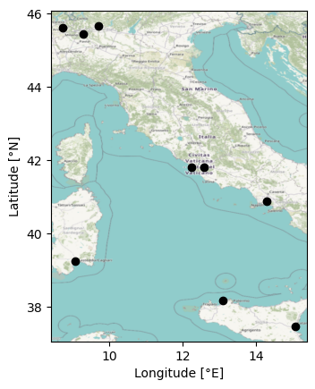
Define the airports#
List the airports and their coordinates.
airports = [
    'Milano Malpensa', 'Milano Linate', 'Bergamo Orio al Serio',
    'Roma Fiumicino', 'Roma Ciampino', 'Napoli Capodichino',
    'Palermo Punta Raisi', 'Catania Fontanarossa', 'Cagliari Elmas'
]
Tip
Enter the locations of your choice here. At least two locations must be defined for the methodology to work.
def to_dataframe(dct):
    idx = pd.Index(airports, name="airport")
    return pd.DataFrame(dct, index=idx, dtype=float)
# List coordinates in the order of the locations from above (°N, °E)
coords = to_dataframe({
    "latitude": [45.63, 45.45, 45.67, 41.80, 41.80, 40.88, 38.18, 37.47, 39.25],
    "longitude": [8.73, 9.28, 9.71, 12.25, 12.59, 14.29, 13.10, 15.07, 9.06]
})

# Check that the coordinates are correctly associated with the airports
coords
| latitude | longitude | |
|---|---|---|
| airport | ||
| Milano Malpensa | 45.63 | 8.73 |
| Milano Linate | 45.45 | 9.28 |
| Bergamo Orio al Serio | 45.67 | 9.71 |
| Roma Fiumicino | 41.80 | 12.25 |
| Roma Ciampino | 41.80 | 12.59 |
| Napoli Capodichino | 40.88 | 14.29 |
| Palermo Punta Raisi | 38.18 | 13.10 |
| Catania Fontanarossa | 37.47 | 15.07 |
| Cagliari Elmas | 39.25 | 9.06 |
fig, ax = plt.subplots(1, 1)
ax.scatter(coords.longitude, coords.latitude, color="k")
ax.set_xlabel("Longitude [°E]")
ax.set_ylabel("Latitude [°N]")
contextily.add_basemap(ax, crs="EPSG:4326", attribution=False)
Component normalization#
The aim of normalization processes is to transform the values of these indicators, which are measured at different scales and in different units, into comparable values considered on a common scale (Master Adapt, 2018). We used the Min-Max method to transform all values to scores in a range from 0 to 1, where the value 0 represents the optimal level, while the value 1 reflects the most critical estimates:
def normalize_columns(df):
    return (df - df.min()) / (df.max() - df.min())
Hazard: temperature and precipitation#
Load the hazard indicator data produced by the hazard assessment notebook and extract the information for the airport locations specified above.
def load_all(files):
    """Load data based on a name-to-file mapping"""
    das = []
    for name, file in files.items():
        path = os.path.join(indicators_path, file)
        if name == "*":
            ds = xr.open_dataset(path)
            das.extend(ds.data_vars.values())
        else:
            da = xr.open_dataarray(path)
            das.append(da.rename(name))
    return xr.merge(das, compat="override")


def extract_points(ds, points):
    """Extract data from the dataset for a set of points"""
    grid = np.column_stack([
        ds["latitude"].values.flatten(),
        ds["longitude"].values.flatten()
    ])
    tree = scipy.spatial.cKDTree(grid)
    _, closest_idx = tree.query(coords.values, k=1)
    idx_y, idx_x = np.unravel_index(closest_idx, ds["latitude"].shape)
    return (
        ds
        .isel(
            x=xr.DataArray(idx_x, dims="airport"),
            y=xr.DataArray(idx_y, dims="airport")
        )
        .drop_vars(["latitude", "longitude"])
        .assign_coords({"airport": coords.index})
        .to_dataframe()
    )
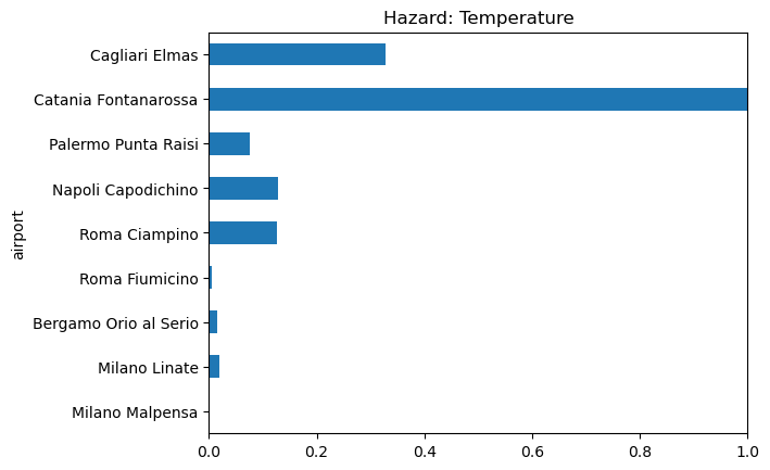
Temperature#
data_temp = load_all({
    "Days Above 35°C": "Temp_DaysAbove35.nc",
    "Days Above 40°C": "Temp_DaysAbove40.nc",
    "Days Above 45°C": "Temp_DaysAbove45.nc",
})
indicators_temp = extract_points(data_temp, coords)
indicators_temp
| Days Above 35°C | Days Above 40°C | Days Above 45°C | |
|---|---|---|---|
| airport | |||
| Milano Malpensa | 0.000000 | 0.000000 | 0.0 |
| Milano Linate | 0.533333 | 0.000000 | 0.0 |
| Bergamo Orio al Serio | 0.433333 | 0.000000 | 0.0 |
| Roma Fiumicino | 0.166667 | 0.000000 | 0.0 |
| Roma Ciampino | 3.400000 | 0.000000 | 0.0 |
| Napoli Capodichino | 3.433333 | 0.000000 | 0.0 |
| Palermo Punta Raisi | 1.266667 | 0.100000 | 0.0 |
| Catania Fontanarossa | 8.933333 | 1.133333 | 0.2 |
| Cagliari Elmas | 6.700000 | 0.266667 | 0.0 |
Combine the indicator columns into a single indicator for the temperature hazard by taking the mean over all columns at each location.
hazard_temp = normalize_columns(indicators_temp).mean(axis=1, skipna=True)

# Quick bar chart of the temperature hazard indicator
hazard_temp.plot.barh(title="Hazard: Temperature", xlim=(0, 1))
<Axes: title={'center': 'Hazard: Temperature'}, ylabel='airport'>
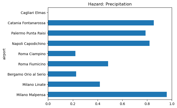
Precipitation#
Repeat the steps for the precipitation indicators:
data_precip = load_all({
    "*": "Precip_return_levels_gumbel.nc",
    "Precip_P99": "Precip_P99.nc",
    "Precip_P999": "Precip_P999.nc"
})
# Remove some left-over coordinates so they don't show up in the indicators table
data_precip = data_precip.drop_vars(["x", "y", "time", "quantile"], errors="ignore")

indicators_precip = extract_points(data_precip, coords)
indicators_precip
| return_period_2_y | return_period_5_y | return_period_10_y | return_period_20_y | return_period_30_y | return_period_50_y | return_period_100_y | return_period_150_y | return_period_200_y | return_period_500_y | Precip_P99 | Precip_P999 | |
|---|---|---|---|---|---|---|---|---|---|---|---|---|
| airport | ||||||||||||
| Milano Malpensa | 77.240410 | 97.857880 | 111.508438 | 124.602386 | 132.135010 | 141.551163 | 154.251877 | 161.657974 | 166.906250 | 183.601303 | 48.059845 | 94.042389 |
| Milano Linate | 56.678417 | 70.069450 | 78.935478 | 87.439987 | 92.332420 | 98.448204 | 106.697311 | 111.507561 | 114.916313 | 125.759735 | 34.706484 | 63.180023 |
| Bergamo Orio al Serio | 49.203640 | 59.805862 | 66.825455 | 73.558823 | 77.432358 | 82.274467 | 88.805618 | 92.614090 | 95.312943 | 103.898109 | 33.550508 | 51.886977 |
| Roma Fiumicino | 50.875408 | 69.739494 | 82.229156 | 94.209549 | 101.101570 | 109.716927 | 121.337532 | 128.113785 | 132.915726 | 148.190964 | 27.939688 | 60.487923 |
| Roma Ciampino | 43.058388 | 56.674309 | 65.689232 | 74.336563 | 79.311157 | 85.529648 | 93.917290 | 98.808327 | 102.274323 | 113.299850 | 26.153749 | 52.537727 |
| Napoli Capodichino | 60.708721 | 85.161652 | 101.351616 | 116.881424 | 125.815338 | 136.983170 | 152.046585 | 160.830429 | 167.055054 | 186.855865 | 35.195312 | 84.431564 |
| Palermo Punta Raisi | 56.251366 | 81.191704 | 97.704376 | 113.543732 | 122.655724 | 134.046158 | 149.409836 | 158.368759 | 164.717453 | 184.912949 | 35.360001 | 88.106552 |
| Catania Fontanarossa | 58.424789 | 85.944069 | 104.164230 | 121.641449 | 131.695663 | 144.263901 | 161.216263 | 171.101578 | 178.106750 | 200.390549 | 26.499609 | 81.429756 |
| Cagliari Elmas | 32.551186 | 44.475163 | 52.369877 | 59.942673 | 64.299118 | 69.744881 | 77.090256 | 81.373528 | 84.408836 | 94.064301 | 17.672501 | 37.748158 |
hazard_precip = normalize_columns(indicators_precip).mean(axis=1, skipna=True)

# Quick bar chart of the precipitation hazard indicator
hazard_precip.plot.barh(title="Hazard: Precipitation", xlim=(0, 1))
<Axes: title={'center': 'Hazard: Precipitation'}, ylabel='airport'>
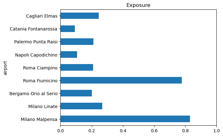
Exposure: air and land side components#
The various airports components, divided into landside and airside areas, were considered as exposed samples in accordance with De Vivo et al. (2022).
The air side components include the structures used for the movement of aircraft, such as runways, taxiways, tower, and aprons:
Air side |
Unit of measurement |
|---|---|
Runways |
Area [m²] |
Taxiways |
Area [m²] |
Tower |
Height [m] |
Apron |
Area [m²] |
The land side components refer to the public access areas such as offices, terminals, airports access systems and parking areas:
Land side |
Unit of measurement |
|---|---|
Terminal |
Area [m²] |
Offices and other buildings |
Area [m²] |
Airport accesses systems |
Area [m²] |
Carparks |
Number |
Define the values for each indicator and airport: (insert None where data is not available)
# Specify the values in the order of the locations defined above
air_land_side_components = to_dataframe({
    'Runways': [470400, 159742, 145530, 396000, 9900, 118260, 292650, 109575, 126000],
    'Taxiways': [250.5, 156, 183, 300, 301, 99, 368, 159, 604],
    'Tower': [80, 47, 30, 56, 60, 40, 25, 12, 28],
    'Apron': [1319000, 387000, 190000, 797250, None, 200000, 148000, 180000, 156000],
    'Terminals': [315000, 85050, 53025, 354300, 20950, 30700, 35400, 43310, 41290],
    'Offices_and_other_buildings': [26715, 13527, 7075, 29520, 5950, 1915, 4180, 6920, 5030],
    'Airport_accesses_systems': [31660, None, None, None, None, None, None, None, None],
    'Carparks': [15000, 3000, 8000, 20100, 1220, 1500, 1364, 1800, 2133]
})

# Check that values are associated correctly to the locations
air_land_side_components
| Runways | Taxiways | Tower | Apron | Terminals | Offices_and_other_buildings | Airport_accesses_systems | Carparks | |
|---|---|---|---|---|---|---|---|---|
| airport | ||||||||
| Milano Malpensa | 470400.0 | 250.5 | 80.0 | 1319000.0 | 315000.0 | 26715.0 | 31660.0 | 15000.0 |
| Milano Linate | 159742.0 | 156.0 | 47.0 | 387000.0 | 85050.0 | 13527.0 | NaN | 3000.0 |
| Bergamo Orio al Serio | 145530.0 | 183.0 | 30.0 | 190000.0 | 53025.0 | 7075.0 | NaN | 8000.0 |
| Roma Fiumicino | 396000.0 | 300.0 | 56.0 | 797250.0 | 354300.0 | 29520.0 | NaN | 20100.0 |
| Roma Ciampino | 9900.0 | 301.0 | 60.0 | NaN | 20950.0 | 5950.0 | NaN | 1220.0 |
| Napoli Capodichino | 118260.0 | 99.0 | 40.0 | 200000.0 | 30700.0 | 1915.0 | NaN | 1500.0 |
| Palermo Punta Raisi | 292650.0 | 368.0 | 25.0 | 148000.0 | 35400.0 | 4180.0 | NaN | 1364.0 |
| Catania Fontanarossa | 109575.0 | 159.0 | 12.0 | 180000.0 | 43310.0 | 6920.0 | NaN | 1800.0 |
| Cagliari Elmas | 126000.0 | 604.0 | 28.0 | 156000.0 | 41290.0 | 5030.0 | NaN | 2133.0 |
As for the hazard, normalize all components and combine into a single indicator for the exposure by taking the mean over all components for each location.
air_land_side_normalized = normalize_columns(air_land_side_components)

# Combine into a single indicator
exposure = air_land_side_normalized.mean(axis=1, skipna=True)

# Quick bar plot of the exposure indicator
ax = exposure.plot.barh(title="Exposure", xlim=(0, 1))
Vulnerability#
Vulnerability reflects “the propensity or predisposition of a system to be adversely affected. It encompasses a variety of concepts and elements including sensitivity or susceptibility to harm and lack of capacity to cope and adapt opportunities, or to respond to consequences” (IPCC, 2022).
Vulnerability is composed of sensitivity and adaptive capacity.
Sensitivity#
Sensitivity is intended as the degree to which the system is (positively or negatively) affected by climate variability or climate change.
Indicator |
Unit of measurement |
|---|---|
Soil Sealing |
Area [%] |
Passenger |
Number |
Building in bad condition |
Number or Absence/Presence |
Age building |
Age |
Air traffic |
Number |
Parking accesses |
Number |
Staff work outside airport |
Number |
Define the sensitivity indicators and their values: (use None where data is not available)
sensitivity_indicators = to_dataframe({
    'Soil_sealing': [1235, 300, 300, 1590, 133, 217, 391, 225, 246],
    'Passengers': [27000000, 7000000, 13857257, 43532573, 5879496, 10860068, 7018087, 10223113, 4747806],
    'Buildings_bad_conditions_or_maintenance': [None, None, None, None, None, None, None, None, None],
    'Age_buildings': [73, 82, 83, 63, 105, 111, 61, 97, 84],
    'Air_traffic': [201050, 85730, 95377, 309783, 52253, 82577, 54243, 73494, 39691],
    'Parking_accesses': [None, None, None, None, None, None, None, None, None],
    'Staff_work': [1997.1, 855.9, 1044, 2363.9, 1013.1, None, 283, 183, 146]
})

sensitivity_normalized = normalize_columns(sensitivity_indicators)
sensitivity_normalized
| Soil_sealing | Passengers | Buildings_bad_conditions_or_maintenance | Age_buildings | Air_traffic | Parking_accesses | Staff_work | |
|---|---|---|---|---|---|---|---|
| airport | |||||||
| Milano Malpensa | 0.756349 | 0.573735 | NaN | 0.24 | 0.597422 | NaN | 0.834618 |
| Milano Linate | 0.114619 | 0.058069 | NaN | 0.42 | 0.170457 | NaN | 0.320078 |
| Bergamo Orio al Serio | 0.114619 | 0.234872 | NaN | 0.44 | 0.206174 | NaN | 0.404888 |
| Roma Fiumicino | 1.000000 | 1.000000 | NaN | 0.04 | 1.000000 | NaN | 1.000000 |
| Roma Ciampino | 0.000000 | 0.029179 | NaN | 0.88 | 0.046510 | NaN | 0.390955 |
| Napoli Capodichino | 0.057653 | 0.157594 | NaN | 1.00 | 0.158783 | NaN | NaN |
| Palermo Punta Raisi | 0.177076 | 0.058535 | NaN | 0.00 | 0.053878 | NaN | 0.061770 |
| Catania Fontanarossa | 0.063143 | 0.141172 | NaN | 0.72 | 0.125154 | NaN | 0.016682 |
| Cagliari Elmas | 0.077557 | 0.000000 | NaN | 0.46 | 0.000000 | NaN | 0.000000 |
Adaptative capacity#
These indicators are defined by the classes reported below and included in De Vivo et al. (2022). If the indicator is present or absent, its value will be 0.9 or 0.1, respectively.
Risk awareness: Initiatives for mitigation to climate change#
Adherence to “NetZero2050” Programme (neutrality 3+)
Certification ISO 50001 and initiatives of “energy saving”
Neutrality 3+ Airport carbon accreditation
Neutrality 4+ Airport carbon accreditation; EP-100 intelligent use of energy from “The Climate Group”- Certification ISO 50001
Level 2 Airport carbon accreditation, environmental improvement program
Commitment to obtaining certfiication
Initiatives for adaptation to climate change#
Efficient drainage system
Present
Insurance policy for extreme events
Absent
Monitoring and alarm system
Present
Present (but alert wind shear)
Absent
Bioinfiltration and permeable pavements
Present
Absent
Risk awareness (and initiatives of mitigation)
Risk management framework
Development of local (Urban) climate change mitigation and adaptation strategies
Sustainability Report 2019
gesap environmental report
Absent
Guidelines for adaptation plan to climate change#
Plan (PACC) and regional strategy for adaptation to climate change
Regional plan under development
Absent
Sustainable Energy and Climate Action Plan (Covenant of Mayors)
Sustainable Energy and Climate Action Plan (Covenant of Mayors) municipality of Catania
Regional climate change adaptation strategy
Class No. |
Description |
Value Range |
Indicator Range (0-1) |
|---|---|---|---|
1 |
Optimal |
0 - 0.2 |
0.1 |
2 |
Quite Positive |
0.2 - 0.4 |
0.3 |
3 |
Neutral |
0.4 - 0.6 |
0.5 |
4 |
Quite Negative |
0.6 - 0.8 |
0.7 |
5 |
Critical |
0.8 - 1 |
0.9 |
Define the adaptive capacity indicators and their values: (use None where data is not available)
adaptive_indicators = to_dataframe({
    'Vegetation_zone': [None, None, None, None, None, None, None, None, None],
    'Initiatives_for_optimization_of_energy ': [0.3, 0.3, 0.3, 0.1, 0.1, 0.3, 0.5, 0.7, 0.7],
    'Green_wall': [0.1, 0.9, 0.9, 0.9, 0.9, 0.9, 0.9, 0.9, 0.9],
    'Green_roof': [0.1, 0.9, 0.9, 0.9, 0.9, 0.9, 0.9, 0.9, 0.9],
    'Heat_resistent_coating': [0.9, 0.9, 0.9, 0.1, 0.9, 0.9, 0.9, 0.9, 0.9],
    'Insurance_policy_for_extreme_events': [0.9, 0.9, 0.9, 0.9, 0.9, 0.9, 0.9, 0.9, 0.9],
    'Guidelines_for_adaptation_climate_change': [0.3, 0.3, 0.3, 0.5, 0.5, 0.9, 0.3, 0.3, 0.3],
    'Evening_departures': [None, None, None, None, None, None, None, None, None]
})

# As defined in the example, the indicators are already normalized into the range [0, 1]
adaptive_normalized = adaptive_indicators
adaptive_normalized
| Vegetation_zone | Initiatives_for_optimization_of_energy | Green_wall | Green_roof | Heat_resistent_coating | Insurance_policy_for_extreme_events | Guidelines_for_adaptation_climate_change | Evening_departures | |
|---|---|---|---|---|---|---|---|---|
| airport | ||||||||
| Milano Malpensa | NaN | 0.3 | 0.1 | 0.1 | 0.9 | 0.9 | 0.3 | NaN |
| Milano Linate | NaN | 0.3 | 0.9 | 0.9 | 0.9 | 0.9 | 0.3 | NaN |
| Bergamo Orio al Serio | NaN | 0.3 | 0.9 | 0.9 | 0.9 | 0.9 | 0.3 | NaN |
| Roma Fiumicino | NaN | 0.1 | 0.9 | 0.9 | 0.1 | 0.9 | 0.5 | NaN |
| Roma Ciampino | NaN | 0.1 | 0.9 | 0.9 | 0.9 | 0.9 | 0.5 | NaN |
| Napoli Capodichino | NaN | 0.3 | 0.9 | 0.9 | 0.9 | 0.9 | 0.9 | NaN |
| Palermo Punta Raisi | NaN | 0.5 | 0.9 | 0.9 | 0.9 | 0.9 | 0.3 | NaN |
| Catania Fontanarossa | NaN | 0.7 | 0.9 | 0.9 | 0.9 | 0.9 | 0.3 | NaN |
| Cagliari Elmas | NaN | 0.7 | 0.9 | 0.9 | 0.9 | 0.9 | 0.3 | NaN |
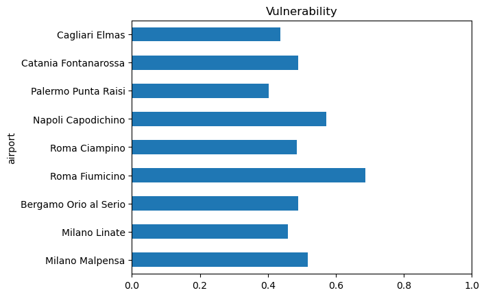
Vulnerability calculation#
Combine the sensitivity and adaptive capacity indicators by taking the mean at each location, then calculate a single vulnerability indicator by taking the mean of these two components.
vulnerability = 0.5 * (
    sensitivity_normalized.mean(skipna=True, axis=1)
    + adaptive_indicators.mean(skipna=True, axis=1)
)

ax = vulnerability.plot.barh(title="Vulnerability", xlim=(0, 1))
Calculate Risk#
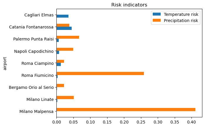
The risk (R) will be computed by multiplication of the three components hazard (H), exposure (E) and vulnerability (V):
R = H * E * V
risk_table = pd.DataFrame.from_dict({
    "Temperature hazard": hazard_temp,
    "Precipitation hazard": hazard_precip,
    "Exposure": exposure,
    "Vulnerability": vulnerability,
    # Calculate the risk by multiplying the components
    "Temperature risk": hazard_temp * exposure * vulnerability,
    "Precipitation risk": hazard_precip * exposure * vulnerability,
})
risk_table.to_csv(os.path.join(indicators_path, f"risk_{region_name}.csv"))
risk_table
| Temperature hazard | Precipitation hazard | Exposure | Vulnerability | Temperature risk | Precipitation risk | |
|---|---|---|---|---|---|---|
| airport | ||||||
| Milano Malpensa | 0.000000 | 0.958177 | 0.830052 | 0.516879 | 0.000000 | 0.411093 |
| Milano Linate | 0.019900 | 0.418003 | 0.266326 | 0.458322 | 0.002429 | 0.051023 |
| Bergamo Orio al Serio | 0.016169 | 0.226971 | 0.200527 | 0.490055 | 0.001589 | 0.022304 |
| Roma Fiumicino | 0.006219 | 0.484378 | 0.776851 | 0.687333 | 0.003321 | 0.258637 |
| Roma Ciampino | 0.126866 | 0.221027 | 0.208675 | 0.484664 | 0.012831 | 0.022354 |
| Napoli Capodichino | 0.128109 | 0.820619 | 0.105080 | 0.571754 | 0.007697 | 0.049303 |
| Palermo Punta Raisi | 0.076675 | 0.786895 | 0.210126 | 0.401793 | 0.006473 | 0.066435 |
| Catania Fontanarossa | 1.000000 | 0.853814 | 0.091670 | 0.489948 | 0.044914 | 0.038348 |
| Cagliari Elmas | 0.328431 | 0.000000 | 0.245209 | 0.437089 | 0.035201 | 0.000000 |
ax = risk_table[["Temperature risk", "Precipitation risk"]].plot.barh(title="Risk indicators")
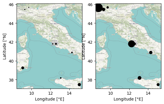
fig, axs = plt.subplots(1, 2)

axs[0].scatter(coords.longitude, coords.latitude, s=risk_table["Temperature risk"]*1000, color="k")
axs[1].scatter(coords.longitude, coords.latitude, s=risk_table["Precipitation risk"]*1000, color="k")

for ax in axs:
    ax.set_xlabel("Longitude [°E]")
    ax.set_ylabel("Latitude [°N]")
    contextily.add_basemap(ax, crs="EPSG:4326", attribution=False)
Classify risk#
To evaluate the risk classes for each of the airport the Quantile Method was used. Classifying each airport in terms of quantile with respect to all other airport taken into account
def classify_risk(risk, classes=["Very Low", "Low", "Medium", "High", "Very High"]):
    return pd.qcut(risk.rank(pct=True), q=len(classes), labels=classes)

risk_classes = pd.DataFrame.from_dict({
    c: classify_risk(risk_table[c]) for c in ["Temperature risk", "Precipitation risk"]
})
risk_classes
| Temperature risk | Precipitation risk | |
|---|---|---|
| airport | ||
| Milano Malpensa | Very Low | Very High |
| Milano Linate | Low | High |
| Bergamo Orio al Serio | Very Low | Very Low |
| Roma Fiumicino | Low | Very High |
| Roma Ciampino | High | Low |
| Napoli Capodichino | High | Medium |
| Palermo Punta Raisi | Medium | High |
| Catania Fontanarossa | Very High | Low |
| Cagliari Elmas | Very High | Very Low |
def highlight_class_column(s):
    """Color the table entries based on the risk classes"""
    colors = {
        "Very Low": "background-color: forestgreen",
        "Low": "background-color: limegreen",
        "Medium": "background-color: yellow",
        "High": "background-color: orange",
        "Very High": "background-color: red; color: white"
    }
    return [colors.get(val, "") for val in s]

risk_classes.style.apply(highlight_class_column, axis=0)
| Temperature risk | Precipitation risk | |
|---|---|---|
| airport | ||
| Milano Malpensa | Very Low | Very High |
| Milano Linate | Low | High |
| Bergamo Orio al Serio | Very Low | Very Low |
| Roma Fiumicino | Low | Very High |
| Roma Ciampino | High | Low |
| Napoli Capodichino | High | Medium |
| Palermo Punta Raisi | Medium | High |
| Catania Fontanarossa | Very High | Low |
| Cagliari Elmas | Very High | Very Low |