Windstorm selection helper#
A workflow from the CLIMAAX Handbook and STORMS GitHub repository.
See our how to use risk workflows page for information on how to run this notebook.
This notebook supports the Hazard assessment for windstorms: select storms based on proximity to a location of interest from a storm track database on CDS: Windstorm tracks and footprints derived from reanalysis over Europe between 1940 to present .
import pathlib
import io
import zipfile

import cdsapi
import earthkit.geo
import earthkit.plots
import numpy as np
import pandas as pd
Preparation#
Define the download folder:
data_dir = pathlib.Path("./STORM_event_raster")
data_dir.mkdir(parents=True, exist_ok=True)

# Where to download storm track dataset:
tracks_zip = data_dir / "windstorm_tracks_cds.zip"
Step 1: Download storm track data#
Retrieve the windstorm tracks from CDS. See the CDS user guide for more information on data access. Skip this step if the file is already available at the location specified in tracks_zip.
URL = "https://cds.climate.copernicus.eu/api"
KEY = None  # put your key if required

client = cdsapi.Client(url=URL, key=KEY)

tracks_zip = client.retrieve("sis-european-wind-storm-reanalysis", {
    "product": "windstorm_track",
    "variable": "all",
    "tracking_algorithm": ["hodges", "tempestextremes"],
    "event_aggregation": "all_events"
}).download(tracks_zip)
Step 2: Read storm track data#
There are two tracking algorithms used to define events in the database. Both report the position of the storm as the locaiton of a mean sea level pressure minimum, but they differ in how they search for the minimum:
"hodges": identify 850 hPa relative vorticity maximum, then find mean sea level pressure minimum within a 5° radius. Captures more small-scale processes and therefore detects more events."tempest_extremes": identify directly by mean sea level pressure minimum.
More information about the tracking algorithms can be found in the dataset’s product user guide.
tracking_algorithm = "hodges"
Read the table of storms for the selected tracking algorithm from the downloaded database:
def select_by_prefix(xs, prefix):
    for x in xs:
        if x.startswith(prefix):
            return x
    raise ValueError(f"No file found for prefix '{prefix}'")


with zipfile.ZipFile(tracks_zip) as archive:
    tracks_file = select_by_prefix(archive.namelist(), f"storm_track-{tracking_algorithm}-")
    with archive.open(tracks_file, "r") as f:
        storms = pd.read_csv(
            io.TextIOWrapper(f),
            index_col=["id", "time"],
            parse_dates=["time"]
        ).sort_index()
Preview of the table:
storms.head()
| latitude | longitude | fg10 | lsm | msl | algorithm | ||
|---|---|---|---|---|---|---|---|
| id | time | ||||||
| 1 | 1940-02-22 00:00:00 | 63.25 | -24.00 | 10.452867 | 0.0 | 98962.875 | hodges |
| 1940-02-22 06:00:00 | 63.50 | -25.00 | 12.599429 | 0.0 | 98905.190 | hodges | |
| 1940-02-22 12:00:00 | 62.75 | -11.25 | 5.919555 | 0.0 | 98809.125 | hodges | |
| 1940-02-22 18:00:00 | 63.00 | -12.00 | 7.741296 | 0.0 | 98755.560 | hodges | |
| 1940-02-23 00:00:00 | 62.75 | -12.25 | 4.190840 | 0.0 | 98655.310 | hodges |
Tip
You can explore the database here or filter it before continuing. For example, you can select only storms that occurred after 2010 with:
storms = storms.loc[storms.index.get_level_values("time") > pd.to_datetime("2010-01-01")]
Step 3: Order storms by distance to location#
Define the coordinates of your location of interest (lat, lon):
lat = 52.012  # °N
lon =  4.359  # °E
Reorder the list of storms such that the geographically closest storms are at the top:
def minimum_distance(track):
    """Shortest distance between the storm track and the location of interest"""
    dist = earthkit.geo.distance.haversine_distance(
        [lat, lon],
        [track.loc[:,"latitude"], track.loc[:,"longitude"]]
    )
    return np.nanmin(dist)

# Add minimum distance of each storm track to the location of interest
# to the table, then sort the table so the closest storms are at the top
sorted_storms = (
    storms
    .join(
        storms
        .groupby("id")
        .apply(minimum_distance)
        .rename("min_distance")
    )
    .sort_values("min_distance")
)
Caveat
The strength of the storm along the track is not taken into account in the minimum_distance function implemented here, only the geographical distance between the chosen location and the storm center at its closest point.
sorted_storm_ids = list(sorted_storms.groupby("id", sort=False).groups.keys())

# The IDs of the ten closest storms
sorted_storm_ids[:10]
[358, 1616, 288, 1526, 1367, 426, 1366, 1484, 1549, 684]
Step 4: Visualize tracks of closest storms#
Display the tracks of the closest storms on a map together with the chosen location:
subplot = earthkit.plots.Map(domain=["North Atlantic", "Europe"])

# Marker for the location of interest
subplot.scatter(x=[lon], y=[lat], marker="*", c="black", s=250, zorder=10)

marker_x = []
marker_y = []
marker_c = []

# Number of storms to show
n = 3

for storm_id in sorted_storm_ids[:n]:
    storm_track = storms.loc[storm_id].sort_index()
    x = storm_track.loc[:,"longitude"].values
    y = storm_track.loc[:,"latitude"].values
    # Line for the track
    subplot.line(x=x, y=y, label=f"Storm ID {storm_id}", zorder=4)
    # Collect track information so storm strength markers can be plotted together
    # with a consistent colorscale
    marker_x.extend(x)
    marker_y.extend(y)
    marker_c.extend(storm_track.loc[:,"msl"] / 100)  # hPa
    n = n - 1
    if n == 0:
        break

# Markers indicating the value of reference variable to represent storm strength
sc = subplot.scatter(x=marker_x, y=marker_y, c=marker_c, marker="o", cmap="Greys_r", zorder=5)

subplot.fig.colorbar(sc, label="storm center mean sea level pressure [hPa]", orientation="horizontal")
subplot.ax.legend()

subplot.land()
subplot.borders()
subplot.gridlines()
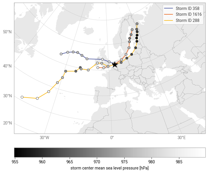
Lower values of mean sea level pressure generally indicate a stronger storm.
Step 5: Find the corresponding storm(s) on CDS#
To download the gridded storm footprint for a storm from the tracks database, the date under which the data has been filed on CDS must be found. It is usually the date at which the storm is first tracked.
storm_id = 358

storms.loc[storm_id]  # enter a storm ID to see the data for the corresponding track
| latitude | longitude | fg10 | lsm | msl | algorithm | |
|---|---|---|---|---|---|---|
| time | ||||||
| 1958-12-09 12:00:00 | 53.25 | -36.00 | 16.655293 | 0.000000 | 98054.375 | hodges |
| 1958-12-09 18:00:00 | 54.75 | -31.75 | 17.521915 | 0.000000 | 97930.000 | hodges |
| 1958-12-10 00:00:00 | 55.50 | -27.75 | 14.142773 | 0.000000 | 97696.625 | hodges |
| 1958-12-10 06:00:00 | 55.75 | -24.25 | 13.544517 | 0.000000 | 97608.560 | hodges |
| 1958-12-10 12:00:00 | 55.00 | -20.50 | 11.378557 | 0.000000 | 97627.625 | hodges |
| 1958-12-10 18:00:00 | 54.00 | -16.25 | 9.302895 | 0.000000 | 97836.560 | hodges |
| 1958-12-11 00:00:00 | 54.25 | -4.50 | 9.535096 | 0.207638 | 98216.875 | hodges |
| 1958-12-11 06:00:00 | 53.25 | 0.50 | 11.224004 | 0.167126 | 98017.190 | hodges |
| 1958-12-11 12:00:00 | 52.50 | 4.00 | 11.516340 | 0.000000 | 98184.375 | hodges |
| 1958-12-11 18:00:00 | 52.00 | 4.25 | 8.077083 | 0.636478 | 98628.940 | hodges |
Use the data selection interface on the CDS website to configure the request interactively or try the configuration generated by the next cell directly in the Hazard assessment for windstorms.
date = storms.loc[storm_id].index.min()

print(f"""
year = '{date.year}'
month = '{date.month:0>2}'
day = '{date.day:0>2}'
""")
year = '1958'
month = '12'
day = '09'
Important
When loading the downloaded storm footprint, confirm that the track_id in the dataset is the same as your expected storm ID.
If not, use the interactive request page on CDS to find data from nearby dates and try these as well.