Exposure datasets

Exposure datasets#

A variety of exposure datasets are available at pan-European scale that can be selected based on the data needs in terms of spatial and temporal resolution and the underlying acquisition or modeling approach. We describe a selected set of exposure datasets, including current exposure and future projections, in more detail below.

A range of population datasets are available, with different spatial and temporal resolutions, such as the satellite-based Global Human Settlement Layer (GHSL) population data GHS-POP, available at $100 m/3 arcsec$ and $1 km/30 arcsec$ from 1975 to 2030 in 5-year time steps. GHS-POP spatially disaggregates census unit-level population numbers with the help of built-up land derived from satellite imagery. Further, WorldPop provides population data in annual time steps for the period 2000-2020 based on a Random Forest modelling approach. GHS-POP and WorldPop are based on the Gridded Population of the World (GPW) (version 4) that have a spatial resolution of 30 arc seconds and a temporal resolution of 5-year time steps from 2000-2020, collected from the national census and population registries. Figure 1 visualizes the three global population datasets for Central Europe.

At the European scale, several population datasets are worth mentioning. The GEOSTAT population grids have a spatial resolution of 1 km and are available for the years 2006, 2011, 2018, 2021. While the years 2011 and 2021 are based on census data, the other years use land cover data and built-up land to disaggregate the population spatially. The Historical Analysis of Natural HaZards in Europe (HANZE) database v2.0 provides population raster data at 100 m spatial resolution for the years 1870-2020, derived from the GEOSTAT data of 2011. On an administrative unit level, i.e. NUTS regions, population data are available from Eurostat and the RDH. An overview of the datasets described in this section can be found in Table 1.

Table 1 Pan-European population datasets with technical specifications and advantages and disadvantages#
Dataset	Spatial scale	Temporal resolution	Spatial resolution	Analysis type	References	Pros	Cons
GHS-POP	Global	1975-2030	100 m, 3 arcsec; 1 km, 30 arcsec	Spatial distribution based on built-up land	European Commission, 2023	Lightly modelled based on census data and Landsat imagery; available in 5-year time steps	Overconcentration of population where built-up land undetected (less problematic in Europe)
WorldPop	Global	2000-2020	3 arcsec, 30 arcsec	Random Forest algorithm	Bondarenko et al., 2020; Stevens et al., 2015	High spatial and temporal resolution	Modelling algorithm based on several input datasets
GPW v4	Global	2000-2020	30 arcsec	National census and population registries	CIESIN, 2018b	Unmodeled	Different spatial and temporal input data
GEOSTAT	Europe	2006, 2011, 2018, 2021	1 km	Derived and modelled from census data	GEOSTAT	Based on census data of 2011 and 2021	No pan-European coverage; 2006 and 2018 modelled
HANZE 2.0	Europe	1870-2020	100 m	Modelled from GEOSTAT 2011	Paprotny & Mengel, 2023	High spatial and temporal resolution	No pan-European coverage
EUROSTAT	Europe	1960-2023	NUTS regions	National census and population registries	EUROSTAT	Consistent across EU countries	No pan-European coverage

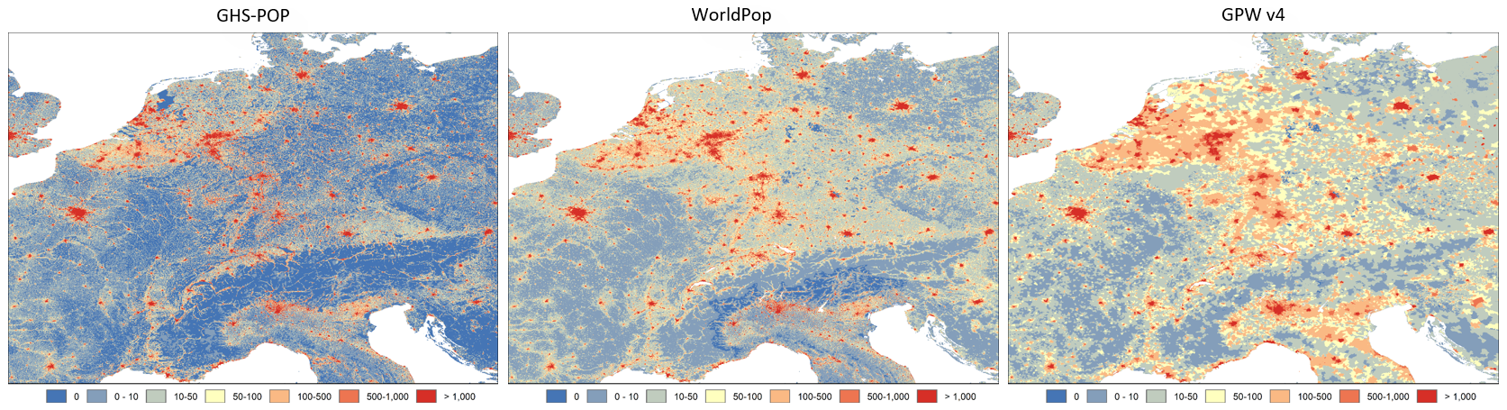
../../_images/ev_data_image2.png — Fig. 10 Spatial population distribution in GHS-POP, WorldPop, and GPW v4#

Several datasets that represent settlements, buildings, infrastructure, and different land uses are available.

GHSL provides raster data of built-up land and volume, residential and non-residential settlement zones (Morphological Settlement Zones), settlement classes, and building height at 2 m to 1 km/ 30 arc seconds spatial resolution and a temporal resolution of five-year time steps from 1975 to 2030 for most datasets. It also provides built-up land data summarized at Local Administrative Unit Level (LAU) for 1975-2020.
Open Street Map (OSM) provides spatial data in vector format (i.e. points, lines, polygons) of e.g. building footprints and types, health and education facilities, energy and telecommunication towers, and roads and railway networks. This crowd-sourced data product is continuously updated by the OSM community.
The Critical Infrastructure Spatial Index (CISI) is based on OSM data and is available in raster format at a spatial resolution of 0.1 decimal degrees.
For assessing the exposure of different land uses, the Europe-wide CORINE land cover data are available for 44 land cover classes at 100 m spatial resolution for the years 1990, 2000, 2006, 2012, and 2018. The CORINE data provide the basis for the higher-detail LUISA land cover map, available for 2012 and 2018 at 50 m spatial resolution. Compared to CORINE, the LUISA Base Map delivers a higher overall spatial detail and finer thematic breakdown of artificial land use/cover categories (17 categories instead of 11 in CORINE). The LUISA Base Map can be used for multiple purposes, and it is more suitable than CORINE for applications requiring fine spatial and/or thematic detail of land use/land cover consistently across Europe, such as land use/cover accounting and modelling. Based on the LUISA land cover map of 2018 combined with OSM data, the European Settlement Map (ESM) was developed at 2 m spatial resolution, including residential versus non-residential buildings.
SPAM is a global crop distribution model covering 42 crops and four different technologies available for 2010 (latest) on a 5 arc-minutes crop-specific grid. The model outputs include both harvested and physical cropland. The Gridded Livestock of the World maps (GLW) show the density of eight different livestock animals in 2010 and 2015 on a 5 arc-minutes animal-specific grid and can be used to represent the exposure of animal husbandry systems. The Global Agro-Ecological Zones (GAEZ) platform provides a range of datasets for agriculture exposure and vulnerability in 2010 values. For instance, the Aggregate Crop Production Value (US$) can be the exposure term in an agricultural drought risk assessment.

Table 2 Pan-European datasets to characterize physical exposure with technical specifications and advantages and disadvantages#
Variable	Dataset	Spatial scale	Temporal resolution	Spatial resolution	References	Pros	Cons
Settlements	GHS-BUILT	Global	1975-2030	From 10 m to 1km/30 arcsec	European Commission, 2023	Global coverage; Different products (e.g. built-up land and volume, building height, residential and non-residential settlements)	Uncommon coordinate reference system: Mollweide
	ESM	Europe	2018	2 m	Szabo et al., 2023	Very high resolution; Distinguishes residential and non-residential buildings	Ukraine missing
Buildings, Infrastructure	OSM	Global	Most recent	Vector data (points, lines, polygons)	OpenStreetMap contributors, 2023	High spatial detail; Good coverage in northern Europe	Working with the data can be cumbersome (e.g. download, selection); Limited coverage in southern Europe
Infrastructure	CISI	Global	2021	0.1 degree	Nirandjan et al., 2022	Input data and final index in raster format; Easy to use (compared to OSM)	Low resolution
Land cover	CORINE	Europe	1990, 2000, 2006, 2012, 2018	100 m	Copernicus Land Monitoring Service, 2018	Relatively long time series	Fewer land cover categories or less spatial detail than LUISA
	LUISA	Europe	2012, 2018	50 m	Pigaiani & Batista e Silva, 2021	17 land cover categories	Ukraine missing; Mixed land use in a cell
	SPAM2010	Global	2010	5 arc minutes	Yu et al., 2020	42 crops available	Low resolution
Livestock density	GLW	Global	2010, 2015	5 arc minutes	Nicolas et al., 2016	8 different animals	Low resolution
Competition on water	Aqueduct v4	Global	1979-2019	Hydrological sub-catchment scale	Kuzma et al., 2023	Global coverage	Scaled for hydrological sub-catchments
Aggregate Crop Production Value	GAEZ	Global	2010	5 arc minutes	Fischer et al., 2021	Global coverage	Low resolution

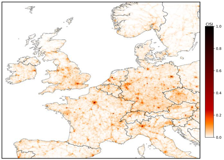
../../_images/ev_data_image6.png — Fig. 11 The CISI for Western Europe (figure adjusted from Nirandjan et al. 2022)#

Table 3 provides an overview of future projections datasets currently available. Future projections of the population until 2100 are available under a range of socioeconomic scenarios, the Shared Socioeconomic Pathways (SSPs) (O’Neill et al., 2017). Publicly available datasets include those of Merkens et al. (2016) and Wang et al. (2022), which are available at a spatial resolution of 30 arc seconds. However, they are based on different modelling approaches and underlying population data used as model input. For instance, the population projections of Merkens et al. 2016 were specifically developed to account for coastal migration processes. Further population projections are available from GHSL at 1 km spatial resolution (Directorate General for Regional and Urban Policy (DG REGIO) of the European Commission, 2020), or from IIASA Global Community Water Model (5 arc minutes) upon request. Projections of future urban land are available for the SSPs until 2100, such as the data of Gao and O’Neill (2020) at 1/8-degree spatial resolution, also downscaled to 1 km, and Chen et al. (2020), available at 30 arc seconds. Additionally, projections of different land uses are available at 30 arc seconds resolution until 2100 (Chen et al., 2022; Zhang et al., 2023), and GHSL provides projections per settlement class (GHS-SMOD) at 1 km resolution until 2070 (Kemper et al., 2022).

Table 3 Pan-European future exposure projections datasets with technical specifications and advantages and disadvantages#
Variable	Scenario	Temporal resolution	Spatial resolution	Acquisition/modelling approach	References	Pros	Cons
Population	SSPs 1-5	2010-2100	30 arcsec	Population growth in coastal, inland, urban, and rural locations	Merkens et al., 2016	Global coverage	Developed with coastal applications in mind
	SSPs 1-5	2020-2100	30 arcsec	Random Forest algorithm	X. Wang et al., 2022	Global coverage	Modelling algorithm based on several input datasets
	SSP-RCP combinations	2015-2100	5 arcmin	Global CWatM	Burek et al., 2020	Global coverage	Dataset not public, but available upon request
Urban land	SSPs 1-5	2015-2100	1 km	Artificial Neural Network algorithm	Chen et al., 2020	Global coverage	Modelling algorithm based on several input datasets
	SSPs 1-5	2000-2100	1/8 decimal degree, 1 km	Monte Carlo simulations	Gao & O’Neill, 2020; Gao & Pesaresi, 2021	Global coverage	Produced at 1/8 decimal degrees and downscaled to 1 km
Land cover	SSP-RCP combinations	2015-2100	30 arcsec	Cellular automata	Chen et al., 2022; Zhang et al., 2023	Based on CMIP6; global coverage	Modelling algorithm based on several input datasets
Competition on water	SSP-RCP combinations	2030-2080	Hydrological sub-catchment scale	Modelled (Aqueduct v4)	Kuzma et al., 2023	Global coverage	Scaled for hydrological sub-catchments

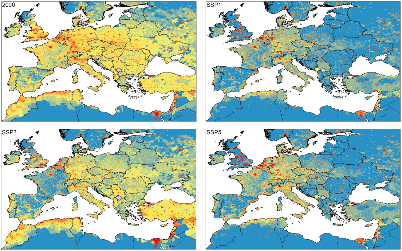
../../_images/ev_data_image7.png — Fig. 12 Population projections by Merkens et al. 2016: Base year (2000) and SSP1, 3, 5 (2100)#

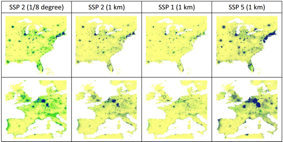
../../_images/ev_data_image8v2.png — Fig. 13 Urban land projections for North America and Europe in 2100 under SSP2, SSP1 and SSP5. Comparison of 1/8 degree spatial resolution (panel 1) to 1 km (panels 2-4) (adjusted from Gao & Pesaresi 2021)#