Heatwave risk under the climate change (Catalunya example)#
A workflow from the CLIMAAX Handbook and HEATWAVES GitHub repository.
See our how to use risk workflows page for information on how to run this notebook.
Description of the assessment#
This notebook combines the hazard Euroheat data with the vulnerability World pop data for the risk estimation for the current and projected climate (rcps 4.5 and 8.5) in the regional resolution for selected EU regions.
Use this workflow to identify regions within your selected area that:
Will be most affected by changes in heatwave occurrence.
Have the highest concentration of vulnerable population groups.
The results provide insight into which areas in your chosen country (or region) may be more impacted by climate change. If some regions are identified as being at a ‘Very High’ risk level, it does not necessarily mean that this risk is the highest among all EU regions. Instead, it indicates that these regions could experience the greatest increase in heat-wave occurrences within the selected country.
Step 1: Preparation work#
Import packages#
In this notebook we will use the following Python libraries:
os - Handling the current working directory.
zipfile - Working with ZIP archive files.
glob - Unix style pathname pattern expansion.
pathlib - File system paths.
geopandas - Geospatial data handling.
cdsapi - Climate Data Store API.
xarray - 2-3D array data handling.
rasterio - NetCDF and raster processing.
numpy - 2-3D array data handling.
rasterio.warp - Raster reprojection and resampling.
rasterstats - Zonal statistics for geospatial raster data.
matplotlib - Data plotting.
rasterio.transform - Coordinate transformations for raster data.
rasterstats - Zonal statistics for geospatial raster data.
mpl_toolkits.axes_grid1 - Data plotting.
matplotlib.colors - Custom colormaps.
import os  # Handling the current working directory.
import zipfile  # Working with ZIP archive files.
import glob  # Unix style pathname pattern expansion.
from pathlib import Path  # File system paths.
import geopandas as gpd  # Geospatial data handling.
import cdsapi  # Climate Data Store API.
import xarray as xr  # 2-3D array data handling.
import rasterio as rio  # NetCDF and raster processing.
import numpy as np  # 2-3D array data handling.
import rasterio  # NetCDF and raster processing.
from rasterio.warp import calculate_default_transform, reproject, Resampling  # Raster reprojection and resampling.
from rasterstats import zonal_stats  # Zonal statistics for geospatial raster data.
import matplotlib.pyplot as plt  # Data plotting.
from rasterio.transform import from_bounds  # Coordinate transformations for raster data.
import rasterstats  # Zonal statistics for geospatial raster data.
from mpl_toolkits.axes_grid1 import make_axes_locatable # Data plotting.
from matplotlib.colors import ListedColormap # Data plotting.
Create a directory structure#
# Define the directory for the flashflood workflow preprocess
#workflow_folder = 'heatwave_risk_projection'
workflow_folder ='heatwave_risk_projection_change'
# Define directories for data and results within the previously defined workflow directory
data_dir = os.path.join(workflow_folder,'data')
results_dir = os.path.join(workflow_folder,'results')
# Check if the workflow directory exists, if not, create it along with subdirectories for data and results
if not os.path.exists(workflow_folder):
    os.makedirs(workflow_folder)
    os.makedirs(os.path.join(data_dir))
    os.makedirs(os.path.join(results_dir))
Step 2: Download the administrative borders#
The risk assessment will be provided to resolve the administrative border area that you choose. It is important to realize that the risk assessment is calculated from the 12x12km hazard data, which means that the selection of the smaller areas will not be appropriate.
Download the shapefile with administrative borders for your country from GADM
Save it to data_dir
Unzip the file to data_dir
Select administrative borders for the zonal statistics#
Tip
You can select different administrative borders for the zonal statistics.
Explore the downloaded data on the data_dir.
Downloaded data will be anding with number 0, 1, 2, 3, 4… depends on selected country
You can change this number in the next step for choosing the different administrative borders for you country (smaller or bigger units)
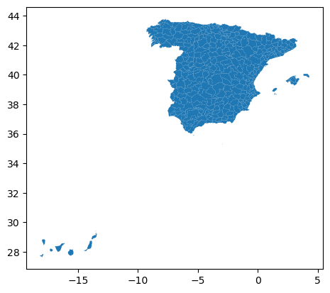
Keep or change the ‘3.shp’ to ‘2.shp’ and you will see the choosen administrative borders plotted below.
# Use glob to find the shapefile ending with '2.shp'
shapefile_pattern = os.path.join(data_dir, '*_3.shp')
shapefile_paths = glob.glob(shapefile_pattern)

# Check if any shapefiles were found and read the first one
if shapefile_paths:
    shapefile_path = shapefile_paths[0]  # Modify this if you need to handle multiple files
    gdf = gpd.read_file(shapefile_path)
    gdf.plot()
else:
    print("no shapefile found")
<Axes: >
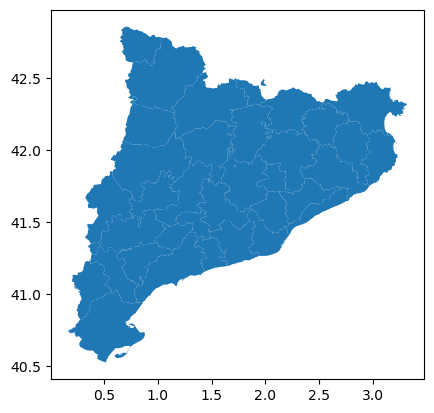
In case you want to select a subregion#
you can select the subregions with this code
if you want to calculate the risk assessment for the whole country then skip this part!!! and continue with the extraction of abounding box
we recommend this approach for bigger countries
select_subregion = 1 # change to 1 to select subregion
subregion_name = 'Cataluña'
# This code can select the subregion e.g.Cataluna
if select_subregion:
    gdf=gdf[gdf["NAME_1"]==subregion_name]
    gdf.plot()
Extract the bounding box for the clipping of the Euroheat and population data#
# Extract the bounding box for the clipping of the Euroheat data
bbox = gdf.total_bounds
# Print the bounding box
print("Bounding Box:", bbox)
Bounding Box: [ 0.15922301 40.52296448 3.32486 42.86132813]
Step 3: Hazard data#
This workflow uses the EuroHEAT hazard data based on the health-related EU-wide definition: For the summer period of June to August, heat waves were defined as days in which the maximum apparent temperature (Tappmax) exceeds the threshold (90th percentile of Tappmax for each month) and the minimum temperature (Tmin) exceeds its threshold (90th percentile of Tmin for each month) for at least two days. The apparent temperature is a measure of relative discomfort due to combined heat and high humidity, developed based on physiological studies on evaporative skin cooling. It can be calculated as a combination of air and dew point temperature.
We use this data to provide information about the projected change in the heatwave occurrence for the near future 2016-2045 and further future 2046-2075
The results are provided in the regional resolution
In the next steps we are using these data together with the vulnerable population data to estimate projected risk levels for the near and further future.
Data download#
In this step we downloading the data from the Copernicus Climate Data Store [source]
URL = "https://cds.climate.copernicus.eu/api"
KEY = None ### put here your key!!!
# Heat waves and cold spells in Europe derived from climate projections
c = cdsapi.Client(url=URL, key=KEY)
c.retrieve(
    'sis-heat-and-cold-spells',
    {
        'variable': 'heat_wave_days',
        'definition': 'health_related',
        'experiment': [
            'rcp4_5', 'rcp8_5',
        ],
        'ensemble_statistic': [
            'ensemble_members_average', 'ensemble_members_standard_deviation',
        ],
        'format': 'zip',
    },
   f"{data_dir}/heat_spells_health_1986_2085.zip")
# This code unzips the downloaded files in your working directory, so they will be ready for computing
# Define zip file's absolute path
zip_path = os.path.join(data_dir, 'heat_spells_health_1986_2085.zip')
# Extract from zip file
with zipfile.ZipFile(zip_path, 'r') as zObject:
    zObject.extractall(path=data_dir)
Extracting the heat occurrence data#
In this step we:
Extracting the heat occurrence values from data
Setting of the Coordinate system
Selecting of the time periods
# This code loads a data form data dir and sets the CRS
hwd45h = xr.open_dataset(f'{data_dir}/HWD_EU_health_rcp45_mean_v1.0.nc', decode_coords='all')
hwd85h = xr.open_dataset(f'{data_dir}/HWD_EU_health_rcp85_mean_v1.0.nc', decode_coords='all')

hwd45h.rio.write_crs("epsg:4326", inplace=True)
hwd85h.rio.write_crs("epsg:4326", inplace=True)

# This code selects a variable for plotting
hwd45h=hwd45h['HWD_EU_health']
hwd85h=hwd85h['HWD_EU_health']
# Select a time period for maximum temperature
# Max T
hw45h=hwd45h.sel(time=slice("1986-01-01", "2015-12-31"))
hw45p1=hwd45h.sel(time=slice("2016-01-01", "2045-12-31"))
hw45p2=hwd45h.sel(time=slice("2046-01-01", "2075-12-31"))

hw85h=hwd85h.sel(time=slice("1986-01-01", "2015-12-31"))
hw85p1=hwd85h.sel(time=slice("2016-01-01", "2045-12-31"))
hw85p2=hwd85h.sel(time=slice("2046-01-01", "2075-12-31"))
Calculation of the mean values for historical and projection periods#
This step calculates the mean values for the selected historical and projections time periods
### Calculates the mean values for the selected time periods and clips data to shp. bbox
# 45 mean
# 1986-2015
hw45hc=hw45h.rio.clip_box(minx=bbox[0], miny=bbox[1], maxx=bbox[2], maxy=bbox[3])
hw45hc= hw45hc.mean(dim='time', skipna=True, keep_attrs=True)
hw45hc.rio.to_raster(raster_path=f'{data_dir}/hw45hc.tif')
# 2016-2045
hw45p1c=hw45p1.rio.clip_box(minx=bbox[0], miny=bbox[1], maxx=bbox[2], maxy=bbox[3])
hw45p1c= hw45p1c.mean(dim='time', skipna=True, keep_attrs=True)
hw45p1c.rio.to_raster(raster_path=f'{data_dir}/hw45p1c.tif')
# 2046-2075
hw45p2c=hw45p2.rio.clip_box(minx=bbox[0], miny=bbox[1], maxx=bbox[2], maxy=bbox[3])
hw45p2c= hw45p2c.mean(dim='time', skipna=True, keep_attrs=True)
hw45p2c.rio.to_raster(raster_path=f'{data_dir}/hw45p2c.tif')
# 85 mean
# 1986-2015
hw85hc=hw85h.rio.clip_box(minx=bbox[0], miny=bbox[1], maxx=bbox[2], maxy=bbox[3])
hw85hc= hw85hc.mean(dim='time', skipna=True, keep_attrs=True)
hw85hc.rio.to_raster(raster_path=f'{data_dir}/hw85hc.tif')
# 2016-2045
hw85p1c=hw85p1.rio.clip_box(minx=bbox[0], miny=bbox[1], maxx=bbox[2], maxy=bbox[3])
hw85p1c= hw85p1c.mean(dim='time', skipna=True, keep_attrs=True)
hw85p1c.rio.to_raster(raster_path=f'{data_dir}/hw85p1c.tif')
# 2046-2075
hw85p2c=hw85p2.rio.clip_box(minx=bbox[0], miny=bbox[1], maxx=bbox[2], maxy=bbox[3])
hw85p2c= hw85p2c.mean(dim='time', skipna=True, keep_attrs=True)
hw85p2c.rio.to_raster(raster_path=f'{data_dir}/hw85p2c.tif')
Relative change of the heatwave occurence#
# This code calculates the relative change in the heatwave occurrence and calculates the zonal statistic based on the imported regions shp.
# Load the raster data
hw45hc = xr.open_dataset(f'{data_dir}/hw45hc.tif')['band_data']
hw45p1c = xr.open_dataset(f'{data_dir}/hw45p1c.tif')['band_data']
hw45p2c = xr.open_dataset(f'{data_dir}/hw45p2c.tif')['band_data']
hw85hc = xr.open_dataset(f'{data_dir}/hw85hc.tif')['band_data']
hw85p1c = xr.open_dataset(f'{data_dir}/hw85p1c.tif')['band_data']
hw85p2c = xr.open_dataset(f'{data_dir}/hw85p2c.tif')['band_data']

# Calculate relative change for RCP 4.5
relative_change_45_p1 = ((hw45p1c - hw45hc) / hw45hc) * 100
relative_change_45_p2 = ((hw45p2c - hw45hc) / hw45hc) * 100

# Calculate relative change for RCP 8.5
relative_change_85_p1 = ((hw85p1c - hw85hc) / hw85hc) * 100
relative_change_85_p2 = ((hw85p2c - hw85hc) / hw85hc) * 100

# Function to ensure the correct shape for raster writing
def save_relative_change_as_raster(relative_change, reference_raster_path, output_path):
    with rasterio.open(reference_raster_path) as src:
        meta = src.meta.copy()
        meta.update(dtype=rasterio.float32, count=1)

        # Ensure relative_change is a 2D array
        relative_change_2d = np.squeeze(relative_change.values)

        with rasterio.open(output_path, 'w', **meta) as dst:
            dst.write(relative_change_2d.astype(rasterio.float32), 1)

# Save the relative change rasters using the correct function
save_relative_change_as_raster(relative_change_45_p1, f'{data_dir}/hw45hc.tif', f'{data_dir}/relative_change_45_p1.tif')
save_relative_change_as_raster(relative_change_45_p2, f'{data_dir}/hw45hc.tif', f'{data_dir}/relative_change_45_p2.tif')
save_relative_change_as_raster(relative_change_85_p1, f'{data_dir}/hw85hc.tif', f'{data_dir}/relative_change_85_p1.tif')
save_relative_change_as_raster(relative_change_85_p2, f'{data_dir}/hw85hc.tif', f'{data_dir}/relative_change_85_p2.tif')

# List of relative change raster files
relative_change_rasters = [
    f'{data_dir}/relative_change_45_p1.tif',
    f'{data_dir}/relative_change_45_p2.tif',
    f'{data_dir}/relative_change_85_p1.tif',
    f'{data_dir}/relative_change_85_p2.tif'
]

# Define the target CRS (WGS84 EPSG:4326)
target_crs = "EPSG:4326"

# Function to reproject raster to a target CRS
def reproject_raster(raster_path, target_crs):
    with rasterio.open(raster_path) as src:
        transform, width, height = calculate_default_transform(
            src.crs, target_crs, src.width, src.height, *src.bounds)
        kwargs = src.meta.copy()
        kwargs.update({
            'crs': target_crs,
            'transform': transform,
            'width': width,
            'height': height
        })

        reprojected_raster_path = raster_path.replace(".tif", "_reprojected.tif")

        with rasterio.open(reprojected_raster_path, 'w', **kwargs) as dst:
            for i in range(1, src.count + 1):
                reproject(
                    source=rasterio.band(src, i),
                    destination=rasterio.band(dst, i),
                    src_transform=src.transform,
                    src_crs=src.crs,
                    dst_transform=transform,
                    dst_crs=target_crs,
                    resampling=Resampling.nearest
                )

    return reprojected_raster_path

# Reproject rasters
reprojected_relative_change_rasters = [reproject_raster(raster, target_crs) for raster in relative_change_rasters]
gdf = gdf.to_crs(target_crs)

# Function to calculate zonal statistics and save to shapefile
def calculate_and_save_zonal_stats(gdf, raster, output_path):
    stats = zonal_stats(gdf, raster, stats="mean", all_touched=True)
    # Handle None values
    mean_values = [round(s['mean']) if s['mean'] is not None else 0 for s in stats]
    gdf_temp = gdf.copy()
    gdf_temp[f"{os.path.basename(raster).replace('.tif', '')}_mean"] = mean_values
    gdf_temp.to_file(output_path)

# Calculate zonal statistics for each reprojected raster
for raster in reprojected_relative_change_rasters:
    output_shapefile_path = f"{data_dir}/{os.path.basename(raster).replace('.tif', '_zonal_stats.shp')}"
    calculate_and_save_zonal_stats(gdf, raster, output_shapefile_path)
Plots the relative change of the heatwave occurrence#
# This code plots the relative change of the heatwave occurrence
# Paths to the reprojected zonal statistics shapefiles
zonal_stats_files = [
    f'{data_dir}/relative_change_45_p1_reprojected_zonal_stats.shp',
    f'{data_dir}/relative_change_45_p2_reprojected_zonal_stats.shp',
    f'{data_dir}/relative_change_85_p1_reprojected_zonal_stats.shp',
    f'{data_dir}/relative_change_85_p2_reprojected_zonal_stats.shp'
]

# Corresponding titles for the plots and filenames for saving
titles = [
    'Heatwave occurrence relative change\nRCP 4.5, 2016-2045 vs 1986-2015',
    'Heatwave occurrence relative change\nRCP 4.5, 2046-2075 vs 1986-2015',
    'Heatwave occurrence relative change\nRCP 8.5, 2016-2045 vs 1986-2015',
    'Heatwave occurrence relative change\nRCP 8.5, 2046-2075 vs 1986-2015'
]

output_filenames = [
    'relative_change_rcp45_2016_2045.shp',
    'relative_change_rcp45_2046_2075.shp',
    'relative_change_rcp85_2016_2045.shp',
    'relative_change_rcp85_2046_2075.shp'
]

# Load all shapefiles into a list of GeoDataFrames
gdfs = [gpd.read_file(file) for file in zonal_stats_files]

# Function to find the column containing 'mean' in the name
def find_mean_column(gdf):
    for col in gdf.columns:
        if 'relative' in col:
            return col
    return None

# Get the column names for all GeoDataFrames
mean_columns = [find_mean_column(gdf) for gdf in gdfs]

# Filter out any None values (in case some GeoDataFrames don't have a 'mean' column)
filtered_gdfs = [(gdf, col) for gdf, col in zip(gdfs, mean_columns) if col is not None]

# Get the global min and max of the relative change values
min_value = min(gdf[col].min() for gdf, col in filtered_gdfs)
max_value = max(gdf[col].max() for gdf, col in filtered_gdfs)

# Define the class intervals and labels for relative change
class_intervals = np.linspace(min_value, max_value, 11).tolist()
class_labels = ['%.1f%%' % val for val in class_intervals]

# Initialize lists to combine GeoDataFrames
combined_gdfs = [gpd.GeoDataFrame() for _ in range(4)]

# Plot each shapefile and save them
fig, axes = plt.subplots(2, 2, figsize=(20, 18))  # 2 rows and 2 columns for the 4 plots
axes = axes.flatten()

for i, (ax, (gdf, col), title, output_filename) in enumerate(zip(axes, filtered_gdfs, titles, output_filenames)):
    # Plot the map
    gdf.plot(column=col, ax=ax, legend=True,
             legend_kwds={'label': "Heatwave occurrence relative change vs 1986-2015 (%)",
                          'orientation': "horizontal",
                          'ticks': class_intervals,
                          'spacing': 'uniform',
                          'format': lambda x, _: class_labels[class_intervals.index(x)] if x in class_intervals else ''},
             vmin=min_value, vmax=max_value, cmap='RdYlGn_r')
    ax.set_title(title)
    ax.axis('off')

    # Append the current GeoDataFrame to the combined list
    combined_gdfs[i] = gdf[[col, 'geometry']].copy()

    # Save each combined GeoDataFrame as a new shapefile
    output_path = os.path.join(results_dir, output_filename)
    combined_gdfs[i].to_file(output_path)

plt.tight_layout()
plt.show()
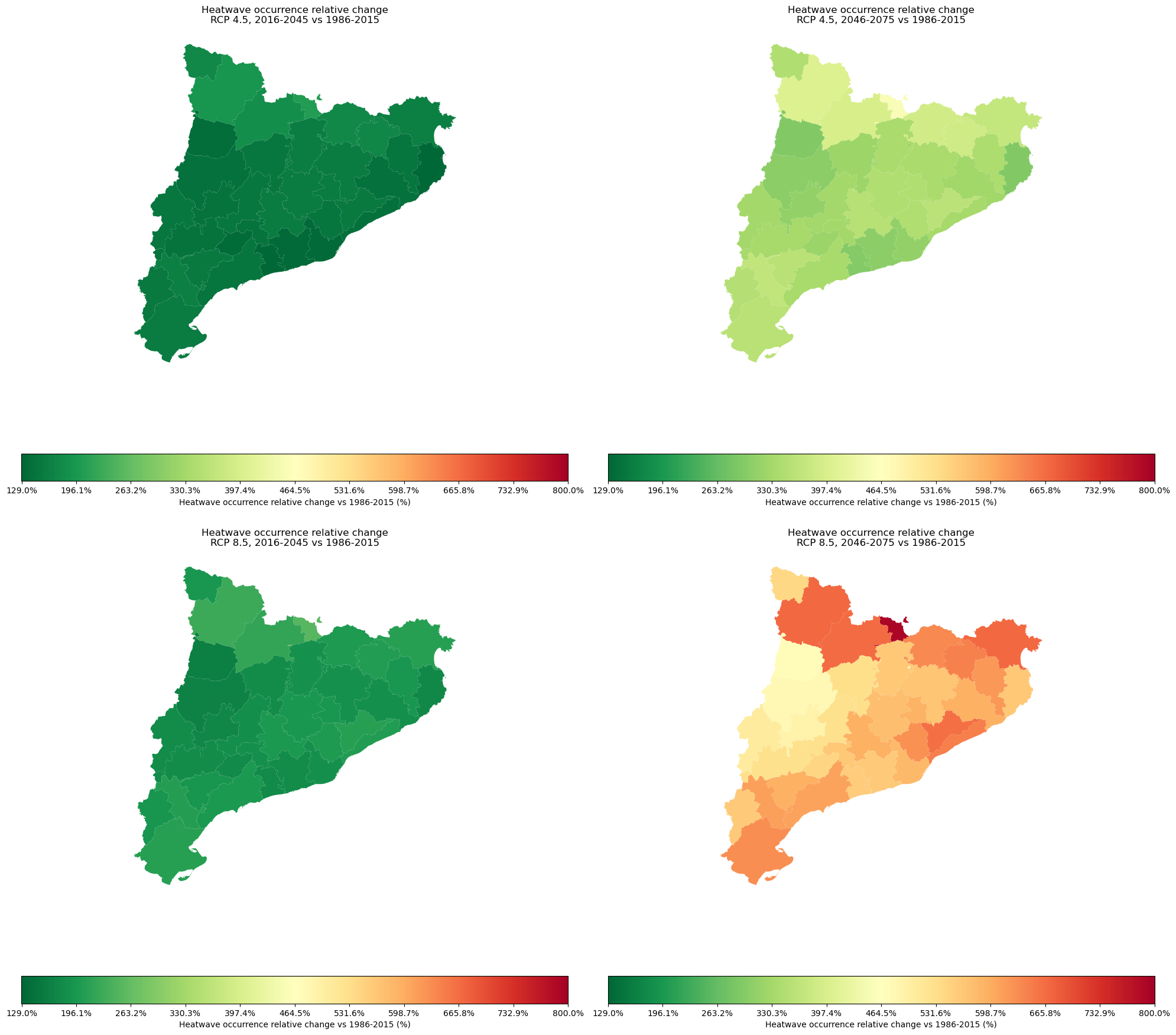
This result represent the relative change in the heatwave occurrence for the selected region vs the heatwave occurence for the reference period 1976-2015.
Magnitude of change in the heatwave occurrence#
This step reclassifies the heatwave occurrence relative change data into 10 equal interval classes. We need this to use the data in the 10+10 risk matrix (in the next steps). The result is the magnitude of change in the heatwave occurrence classified from 1 to 10 (1-very low change, 10-very high change). See the picture above for a percentual expression.
# This code reclassifies the heatwave occurrence relative change data in to 10 equal intervals

# Paths to the shapefiles
shapefiles = [
    f'{results_dir}/relative_change_rcp45_2016_2045.shp',
    f'{results_dir}/relative_change_rcp45_2046_2075.shp',
    f'{results_dir}/relative_change_rcp85_2016_2045.shp',
    f'{results_dir}/relative_change_rcp85_2046_2075.shp'
]

# Corresponding titles for the plots
titles = [
    'Reclassified heatwave occurrence relative change \nRCP 4.5, 2016-2045 vs 1986-2015',
    'Reclassified heatwave occurrence relative change \nRCP 4.5, 2046-2075 vs 1986-2015',
    'Reclassified heatwave occurrence relative change \nRCP 8.5, 2016-2045 vs 1986-2015',
    'Reclassified heatwave occurrence relative change \nRCP 8.5, 2046-2075 vs 1986-2015'
]

# Output filenames for reclassified shapefiles
output_filenames = [
    f'{results_dir}/reclassified_relative_change_rcp45_2016_2045.shp',
    f'{results_dir}/reclassified_relative_change_rcp45_2046_2075.shp',
    f'{results_dir}/reclassified_relative_change_rcp85_2016_2045.shp',
    f'{results_dir}/reclassified_relative_change_rcp85_2046_2075.shp'
]

# Function to find the column containing 'relative' in the name
def find_relative_column(gdf):
    for col in gdf.columns:
        if 'relative' in col:
            return col
    return None

# First, determine the global min and max across all shapefiles
global_min = np.inf
global_max = -np.inf

for shapefile_path in shapefiles:
    gdf_shp = gpd.read_file(shapefile_path)
    relative_col = find_relative_column(gdf_shp)
    if relative_col:
        min_value = gdf_shp[relative_col].min()
        max_value = gdf_shp[relative_col].max()
        global_min = min(global_min, min_value)
        global_max = max(global_max, max_value)

# Print the global minimum and maximum values
print(f"Global Minimum Relative Change: {global_min}%")
print(f"Global Maximum Relative Change: {global_max}%")

# Define the class intervals based on the global min and max
class_intervals = np.linspace(global_min, global_max, 11)

# Create a 2x2 plot grid
fig, axes = plt.subplots(2, 2, figsize=(20, 16))  # 2 rows, 2 columns

# Flatten the axes array to easily iterate over it
axes = axes.flatten()

# Process each shapefile with the determined class intervals
for i, (shapefile_path, title, output_path) in enumerate(zip(shapefiles, titles, output_filenames)):
    # Load the shapefile
    gdf_shp = gpd.read_file(shapefile_path)

    # Identify the column containing the relative change
    relative_col = find_relative_column(gdf_shp)

    if relative_col is None:
        raise ValueError(f"No 'relative' column found in the GeoDataFrame for {shapefile_path}.")

    # Reclassify the data according to the global class intervals
    gdf_shp['class'] = np.digitize(gdf_shp[relative_col], class_intervals, right=True)

    # Print the unique classes to check the distribution
    print(f"Unique classes in {shapefile_path}: {gdf_shp['class'].unique()}")

    # Plot the reclassified data on the corresponding subplot
    gdf_shp.plot(column='class', ax=axes[i], legend=True,
             legend_kwds={
                 'label': "Magnitude of change vs 1986-2015",
                 'orientation': "horizontal",
                 'ticks': np.arange(1, 11),  # Set ticks from 1 to 10
                 'format': lambda x, _: f'{int(x)}'  # Format ticks as integers
             },
             cmap='RdYlGn_r',
             vmin=1, vmax=10)  # Ensure color mapping from 1 to 10

    axes[i].set_title(title)
    axes[i].axis('off')

    # Save the reclassified shapefile
    gdf_shp.to_file(output_path)

# Adjust layout
plt.tight_layout()
plt.show()
Global Minimum Relative Change: 129%
Global Maximum Relative Change: 800%
Unique classes in heatwave_risk_projection_change\results/relative_change_rcp45_2016_2045.shp: [2 1 0]
Unique classes in heatwave_risk_projection_change\results/relative_change_rcp45_2046_2075.shp: [5 4 3]
Unique classes in heatwave_risk_projection_change\results/relative_change_rcp85_2016_2045.shp: [2 1]
Unique classes in heatwave_risk_projection_change\results/relative_change_rcp85_2046_2075.shp: [10  7  8  9  6]
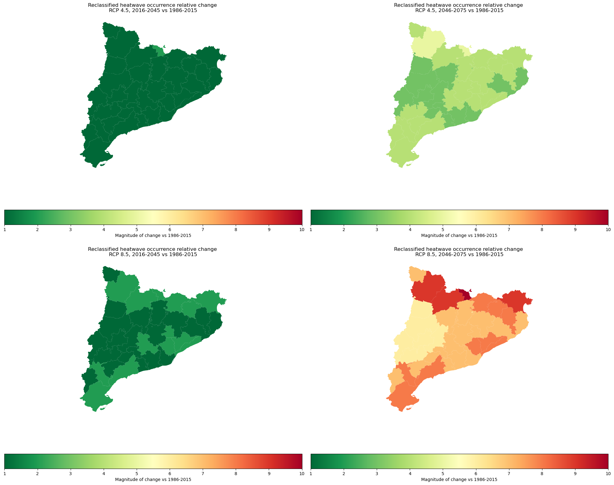
The picture above represents the magnitude of the potential projected increase of the heatwave occurrence among the selected regions from 1 to 10 (1-very low change, 10-very high change)
Step 4: Vulnerable population data#
In this workflow, we use vulnerable population data to identify regions with the highest concentration of vulnerable groups, categorized as ‘Very High.’ If regions are classified as ‘Very Low,’ it does not imply that vulnerable groups are absent; rather, it indicates that their concentration is lower compared to the selected regions.
Go to the Worldpop Hub (DOI: 10.5258/SOTON/WP00646) to access population data:
Enter a country in the search box at the top right of the table. You will find entries valid for different years.
Pick a year (choose the most recent if unsure) and click on Data & Resources next to the corresponding entry.
Download the maps for the most vulnerable groups of the population. This is done by downloading the relevant files from the Data files section of the entry selected above. The data files have names according to the following pattern:
<countrycode>_<sex>_<age>_<year>.tif. For example,svk_m_1_2020.tifcontains data forsvk= Slovakiam= male (please download both male and female (f))1= 1 to 5 years of age, download also for 65, 70, 75, 802020= age structures in 2020
Place the files in the data_dir where you create a folder
population.
When you download all these maps to the Heat-workflow data folder, you can use this code for data handling:
in the first step we load all the maps of the critical population
then we calculate the sum of the vulnerable population from each of the maps
we classified the maps into 10 groups (equal intervals)
plot it next to a map of overheated areas.
Extraction of the data#
Extract the vulnerable population data and sum values for all vulnerable groups of population
# Open all downloaded population files
pop = xr.open_mfdataset(
    os.path.join(data_dir, "population", '*.tif'),
    chunks="auto",
    concat_dim="band",
    combine="nested"
)

# Cut to the region of interest based on the provided shapefile
pop = pop.rio.clip_box(*gdf.total_bounds, crs=gdf.crs)
# Sum over all files at every gridpoint
pop = pop.sum(dim="band", skipna=True, keep_attrs=True)
# Write summed vulnerable population to disk
pop["band_data"].rio.to_raster(raster_path=f'{data_dir}/pop_sum.tif')
Reclassifies the vulnerable population data and calculates the zonal statistics#
Reclassify the vulnerable population data to 10 equal interval groups fo the use in the 10+10 risk matrix with the projected magnitude of change in the heatwave occurrence.
# this code reclassify the vulnerable population data to 10 equal interval and calculates the zonal statistic for selected regions
# Load the shapefile
if select_subregion:
    gdf=gdf[gdf["NAME_1"]==subregion_name]
regions = gdf

# Load the raster data
raster_path = os.path.join(data_dir, 'pop_sum.tif')
with rasterio.open(raster_path) as src:
    raster_data = src.read(1)
    transform = src.transform
    crs = src.crs
    nodata_value = -999  # Specify a nodata value

# Mask out values <= 1
#raster_data = np.where(raster_data > 1, raster_data, np.nan)

# Save the masked raster to a temporary file to use with rasterstats
masked_raster_path = os.path.join(data_dir, 'masked_pop_sum.tif')
with rasterio.open(
    masked_raster_path, 'w',
    driver='GTiff',
    height=raster_data.shape[0],
    width=raster_data.shape[1],
    count=1,
    dtype=rasterio.float32,
    crs=crs,
    transform=transform
) as dst:
    dst.write(raster_data, 1)

# Calculate the zonal statistics
stats = rasterstats.zonal_stats(regions, masked_raster_path, stats="mean", geojson_out=True)
regions_stats = gpd.GeoDataFrame.from_features(stats)

# Extract the mean density values
if 'mean' in regions_stats.columns:
    regions_stats['mean_density'] = regions_stats['mean']
else:
    regions_stats['mean_density'] = regions_stats['properties'].apply(lambda x: x['mean'])

# Determine the class intervals based on the density
num_classes = 10
class_intervals = np.linspace(regions_stats['mean_density'].min(), regions_stats['mean_density'].max(), num_classes + 1)

# Classify the densities
def classify_density(density, class_intervals):
    for i in range(len(class_intervals) - 1):
        if class_intervals[i] <= density < class_intervals[i + 1]:
            return i + 1
    return num_classes

regions_stats['density_class'] = regions_stats['mean_density'].apply(lambda x: classify_density(x, class_intervals))

# Merge with original regions to retain 'NAME_2'
regions_stats = regions_stats.merge(regions[['NAME_2', 'geometry']], on='geometry')

# Save the results to a new shapefile
output_shapefile_path = os.path.join(results_dir, 'population_classified_regions.shp')
regions_stats.to_file(output_shapefile_path)
Plots the zonal statistics for the vulnerable population data#
# Load the classified regions shapefile
classified_shapefile_path = f'{results_dir}/population_classified_regions.shp'
classified_regions = gpd.read_file(classified_shapefile_path)
# Define a colormap similar to the new approach (use a sequential colormap that reflects a gradient change)
cmap = plt.get_cmap("RdYlGn_r")  # You can change this to any preferred colormap that fits the data's range and distribution
# Create a figure and axes
fig, ax = plt.subplots(1, 1, figsize=(10, 8))
# Create a colorbar using make_axes_locatable to replicate a similar style
divider = make_axes_locatable(ax)
cax = divider.append_axes("right", size="5%", pad=0.1)
# Plot the classified regions using the 'density_cl' column
classified_regions.plot(
    column='density_cl',  # Use the appropriate column name for classification
    cmap=cmap,
    linewidth=0.8,
    ax=ax,
    edgecolor='0.8',
    legend=False
)
# Create a ScalarMappable and colorbar with custom ticks and labels
sm = plt.cm.ScalarMappable(cmap=cmap, norm=plt.Normalize(vmin=1, vmax=10))
sm._A = []  # Empty array for the scalar mappable
# Define ticks and labels for the colorbar
cbar = fig.colorbar(sm, cax=cax, ticks=[1, 3.25, 5.5, 7.75, 10])
cbar.ax.set_yticklabels(['Very Low', 'Low', 'Medium', 'High', 'Very High'], size=10)
# Set plot title and labels to match the new approach style
ax.set_title('Classified Regions by vulnerable population density', fontsize=15)
ax.set_xlabel('Longitude', fontsize=12)
ax.set_ylabel('Latitude', fontsize=12)
# Show the plot
plt.show()
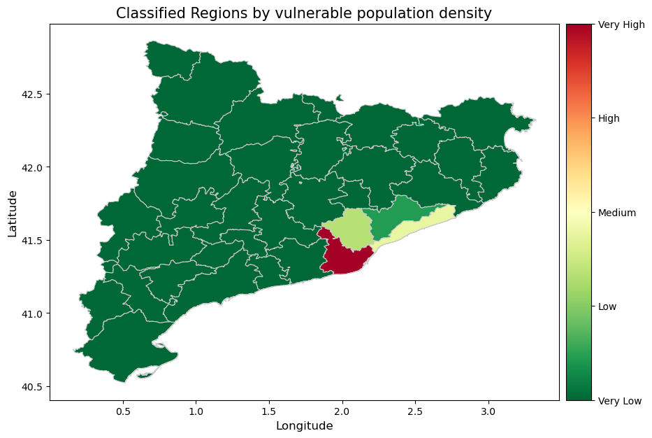
The picture above provides information about the concentration of the vulnerable groups in the population of the Catalunya regions.
Step 5: Estimation of magnitude of heatwave risk change for the vulnerable population#
For the risk estimation we used the 10x10 risk matrix, which combines the heatwave occurence hazard data with vulnerable population data

Calculate the risk values based on the risk matrix#
Combine the magnitude of change in the heatwave occurrence with the vulnerable population density.
Combine the reclassified hazard and vulnerable population data to highlight each region’s risk level.
# This code calculates the sum of the magnitude of change in the heatwave occurrence + vulnerable population density
# Paths to the shapefiles
zonal_stats_paths = [
    ('reclassified_relative_change_rcp45_2016_2045.shp', 'class'),
    ('reclassified_relative_change_rcp45_2046_2075.shp', 'class'),
    ('reclassified_relative_change_rcp85_2016_2045.shp', 'class'),
    ('reclassified_relative_change_rcp85_2046_2075.shp', 'class')
]

classified_regions_path = os.path.join(results_dir, 'population_classified_regions.shp')

# Load the classified regions shapefile
classified_regions = gpd.read_file(classified_regions_path)

# Check if CRS is defined for classified regions, and set it if missing
if classified_regions.crs is None:
    classified_regions.set_crs(epsg=4326, inplace=True)

crs_classified = classified_regions.crs

for file_name, column_name in zonal_stats_paths:
    # Load the zonal stats shapefile
    zonal_stats_path = os.path.join(results_dir, file_name)
    zonal_gdf = gpd.read_file(zonal_stats_path)

    # Check if CRS is defined for zonal stats and set it if missing
    if zonal_gdf.crs is None:
        zonal_gdf.set_crs(epsg=4326, inplace=True)

    # Check CRS and reproject if necessary
    if zonal_gdf.crs != crs_classified:
        zonal_gdf = zonal_gdf.to_crs(crs_classified)

    # Merge the columns
    merged_gdf = classified_regions.copy()
    merged_gdf[column_name] = zonal_gdf[column_name]
    merged_gdf['sum_class'] = merged_gdf['density_cl'] + merged_gdf[column_name]

    # Save the resulting shapefile
    output_path = os.path.join(results_dir, f'sum_class_{file_name}')
    merged_gdf.to_file(output_path)
    print(f"Saved {output_path}")

print("All shapefiles with sum_class created successfully.")
Saved heatwave_risk_projection_change\results\sum_class_reclassified_relative_change_rcp45_2016_2045.shp
Saved heatwave_risk_projection_change\results\sum_class_reclassified_relative_change_rcp45_2046_2075.shp
Saved heatwave_risk_projection_change\results\sum_class_reclassified_relative_change_rcp85_2016_2045.shp
Saved heatwave_risk_projection_change\results\sum_class_reclassified_relative_change_rcp85_2046_2075.shp
All shapefiles with sum_class created successfully.
Plot the risk map#
# List of the zonal statistics shapefiles
zonal_stats_files = [
    'sum_class_reclassified_relative_change_rcp45_2016_2045.shp',
    'sum_class_reclassified_relative_change_rcp45_2046_2075.shp',
    'sum_class_reclassified_relative_change_rcp85_2016_2045.shp',
    'sum_class_reclassified_relative_change_rcp85_2046_2075.shp'
]

# Corresponding titles for the plots
titles = [
    'Relative change of Heatwave risk to vulnerable population groups\nRCP 4.5, 2016-2045 vs 1986-2015',
    'Relative change of Heatwave risk to vulnerable population groups\nRCP 4.5, 2046-2075 vs 1986-2015',
    'Relative change of Heatwave risk to vulnerable population groups\nRCP 8.5, 2016-2045 vs 1986-2015',
    'Relative change of Heatwave risk to vulnerable population groups\nRCP 8.5, 2046-2075 vs 1986-2015'
]

# Load all shapefiles into a list of GeoDataFrames
gdfs = [gpd.read_file(os.path.join(results_dir, file)) for file in zonal_stats_files]

# Get the global min and max of the 'sum_class' values
min_value = min(gdf['sum_class'].min() for gdf in gdfs)
max_value = max(gdf['sum_class'].max() for gdf in gdfs)

# Define the class intervals and labels
class_intervals = [1, 5.75, 10.5, 15.25, 20]
class_labels = ['Very Low', 'Low', 'Medium', 'High', 'Very High']

# Plot each shapefile
fig, axes = plt.subplots(2, 2, figsize=(20, 18))  # Changed to 2 rows and 2 columns
axes = axes.flatten()

for ax, gdf, title in zip(axes, gdfs, titles):
    plot = gdf.plot(column='sum_class', ax=ax, legend=True,
                    legend_kwds={'label': "Risk",
                                 'orientation': "horizontal",
                                 'ticks': class_intervals,
                                 'spacing': 'uniform',
                                 'format': lambda x, _: class_labels[class_intervals.index(x)] if x in class_intervals else ''},
                    vmin=1, vmax=20, cmap='RdYlGn_r')
    ax.set_title(title)
    ax.axis('off')

# Adjust the color bar manually to fit the intervals and labels
cbar = fig.get_axes()[-1]

plt.tight_layout()
plt.show()
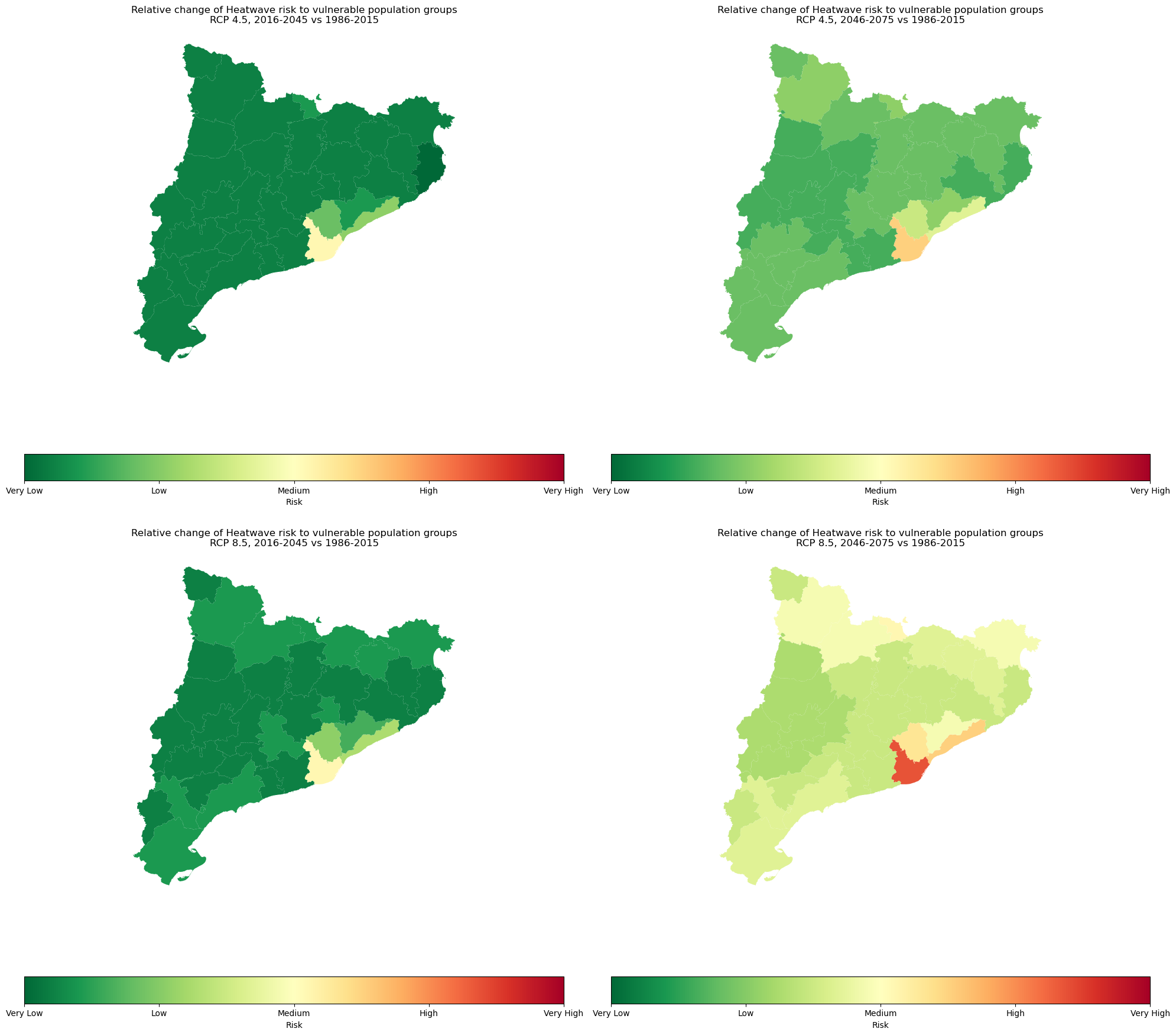
The picture above shows the potential projected increase of the heatwave risk to vulnerable population groups among the selected regions. This result is based on the combination of the projected magnitude of change in the heatwave occurrence with the distribution of the vulnerable groups of the population.
Conclusion#
The results of this workflow provide insights into the relative changes in heatwave occurrence, the distribution of vulnerable population groups, and the projected heatwave risk for these vulnerable groups.
These findings help to better understand the projected magnitude of change in heatwave occurrence and highlight areas with a higher concentration of vulnerable population groups. Additionally, this workflow demonstrates the methodology for combining these two sets of information using a 10x10 risk matrix.
It is important to note that the level of risk is dependent on the area selected at the beginning of the analysis. This means that the risk level only reflects differences between the chosen regions.
All results are save in the working directory results_dir and you can you other free available GIS software (e.g. [QGIS]) to closely explore the data
References#
Climate adapt (2007), EuroHEATonline heat-wave forecast [2024-06-17]
Copernicus Climate Data Store (2019), Heat waves and cold spells in Europe derived from climate projections, [2024-06-17].
GADM (2018), shapefiles of the European regions [2024-06-20]
QGIS.org (2024). QGIS Geographic Information System. Open Source Geospatial Foundation Project. http://qgis.org [2024-06-20]