Exploring future climate projections and plausibility#
Climate models are often used in climate risk assessments. They simulate future changes in weather patterns under different emission scenarios. The resulting estimates of future climate conditions are often called climate projections. These projections help gain insight into what the world of tomorrow can look like in terms of average temperature, heavy rainfall estimates, heatwave days, dry spell duration, and much more.
However, since there are many climate models that each provide their own projections, we will discuss how we can retrieve information from these numbers and how we can explore a representative scenario range.
Theory#
Many models, many different projections#
From a set of climate model runs many different climate conditions are projected. One reason for this variation is the difference in emissions in the atmosphere that cause global warming. Another reason is that even within a similar emission scenario, different models behave differently because they represent the Earth’s climate system differently. Since there is imperfect knowledge, models have varying assumptions, simplifications and parameters, leading to varying outcomes. Lastly, there is what we call internal variability. This means that even for a projection with a similar emission scenario and the same climate model, there can be a different projection. This is due to the natural randomness of the weather. This randomness is especially present when considering changes at short time scales.
For example, in the mid-century, some models might project significant droughts in a specific region, while another projection might show limited change in the same region. However, both are plausible scenarios. Here, we show to gain insight into these these uncertainties.
Emission scenarios#
One way to analyse the group of projections from GCMs is by averaging the projections per emission scenario. Emission scenarios like RCPs (Representative Concentration Pathways) and SSPs (Shared Socioeconomic Pathways) are used to predict how the climate will change in the future due to human greenhouse gas emissions. These scenarios are often found in climate risk datasets and also used often in the CLIMAAX workflows. A key strength of these scenarios is their focus on human-caused changes. To make the predictions more reliable, scientists average the results from multiple climate models, which helps smooth out uncertainties and natural climate variations.
However, averaging also dampens the change signal. Different climate models predict different and sometimes opposite changes in temperature and rainfall patterns, even with the same emissions levels, leading to a wide range of possible outcomes. By averaging the model projections, some important details can get lost.
What are SSPs?
Future climate projections are formulated around Shared Socioeconomic Pathways (SSPs), which are scenarios of projected socioeconomic global changes. The set of scenarios is presented in the figure below. The lower SSP numbers represent more sustainable developments and a larger number of implemented climate mitigation measures, whereas SSP5 represents a continuation of former practices leading to the highest greenhouse gas emissions and most severe impacts of climate change.
The full scenario names are identified by a name in the form of SSPx-y, where SSPx is the socioeconomic pathway used to model the scenario and y is the so-called ‘radiatative forcing’ (in W/m2) resulting from the greenhouse gas emissions under the socio-economic scenario in the year 2100. The higher the greenhouse gas concentrations in the atmosphere, the larger both the radiative forcing and the temperature increase (IPCC, 2021).
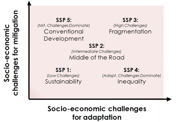
Fig. 17 Shared Socioeconomic Pathways mapped in the challenges to mitigation/adaptation space (copied from O’Neill et al., 2017).#
Global warming levels
Global Warming Levels (GWLs) are another way of aggregating model projections. Here, we don’t use emission scenarios as the main identifier, but we take the level of change for given global temperature warming levels such as 1.5°C or 2°C. So, for each model we assess when this given GWL is reached, we retrieve the climate model data and assess the climate change signal for all climate variables of interest. This offers a simpler, outcome-focused way to assess climate change impacts. Instead of focusing on uncertain emissions pathways, GWLs allow us to directly explore the risks associated with different levels of warming, which can be more intuitive for planning and decision-making. This approach sidesteps some of the uncertainties tied to future emissions and helps focus on the temperature outcomes that matter most for adaptation. However, as with emission scenarios, uncertainty remains in how other climate variables respond to a level of global warming. .
Exploring Plausibility#
Because projections can vary widely, it is important to explore the range of of projections, i.e. the plausibility. By doing so we gain a more comprehensive understanding of what could happen in a specific region, going beyond the limitations of model averages and single projections. We gain deeper insights into changes in local vulnerabilities. The added granularity of projections can help decision-makers planning more robustly and still cost-effective for a wider range of future scenarios.
CMIP vs CORDEX
When exploring future climate scenarios, you can use for example CMIP6 or CORDEX data. CMIP6 provides data from the latest global climate model runs. CORDEX is a downscaled version of the older CMIP5 data, which tries to capture small-scale variations better. CORDEX can, therefore, be more useful for local and regional studies. CMIP6 has a resolution of 50 to 100km, while CORDEX can reach a resolution of 12 to 25km, making it more applicable to the regional scale.
Excercise#
But how do we put the knowledge provided above into practice? In this exercise, we will explore the range of potential climate futures for your region and help you discover why these changes occur. These plausible changes are highlighted using individual climate model projections that can be reviewed for future weather patterns in one of the other CLIMAAX risk workflows. To help guide you we have worked out and example. We introduce each of the steps using a real-life example in Latvia. Be sure to expand the Latvian example section if you want to see how we execute and interpret each step for a real study.
This page will go through the following steps:
Define locally relevant climatic impact drivers
Collect observation trends
Collect simulation trends
Look into IPCC reports why this occurs
Advanced steps
Latvian example
For our example, we take the Lielupe basin, covering parts of Lithuania and Latvia. For Latvia, the basin has been characterised as a flood zone of national importance. See the figure below for an indication of the flood challenges in the region. Information on how these floods will develop in the future is of significant value as more and more adaptation plans and investments will need to be made as we head into the mid-century.
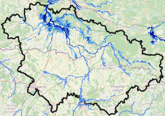
Fig. 18 Flood extent in the Lielupe Basin#
1. Define locally relevant climatic impact drivers#
Begin by identifying the specific climatic conditions that contribute to your climate-related challenge. The more specific you can be, the easier it will be to track changes and predict future hazards. Below is a set of key climate variables that can be explored on a yearly basis or for specific seasons.
Mean Temperature
Minimum Temperature
Minimum of Minimum Temperature
Frost Days
Heating Degree Days
Maximum Temperature
Maximum of Maximum Temperature
Days with Temperature > 35°C
Days with Temperature > 35°C (Bias Corrected)
Days with Temperature > 40°C
Days with Temperature > 40°C (Bias Corrected)
Cooling Degree Days
Total Precipitation
Maximum 1-Day Precipitation
Maximum 5-Day Precipitation
Consecutive Dry Days
Standardized Precipitation Index (6 months)
Total Snowfall
Surface Wind Speed
Latvian example
Flooding in Latvia has two main flood drivers in Latvia, flooding is primarily driven by two factors. One is the snowpack accumulated in winter that rapidly melts and the melt water flows into rivers during spring. Another driver is spring precipitation, which saturates the soil and when this soil is confronted with extra rainfall, the region starts to flood.
To analyse developments for the two flood mechanisms we select the following climate impact drivers:
Average precipitation March till May
Snowfall in December till February
2. Collect observation trends from interactive climate atlas#
To get a better understanding of what climate trend we can expect we will explore what climate trend is already observed. But before we begin we need to define our region using the IPCC climate zones. The IPCC divides Europe into four climatic zones. These zones are based on areas with similar climate typologies. For each of these zones, climate projection statistics are available.
NEU - Northern Europe
WCE - West and Central Europe
MED - Mediterranean
EEU - Eastern Europe
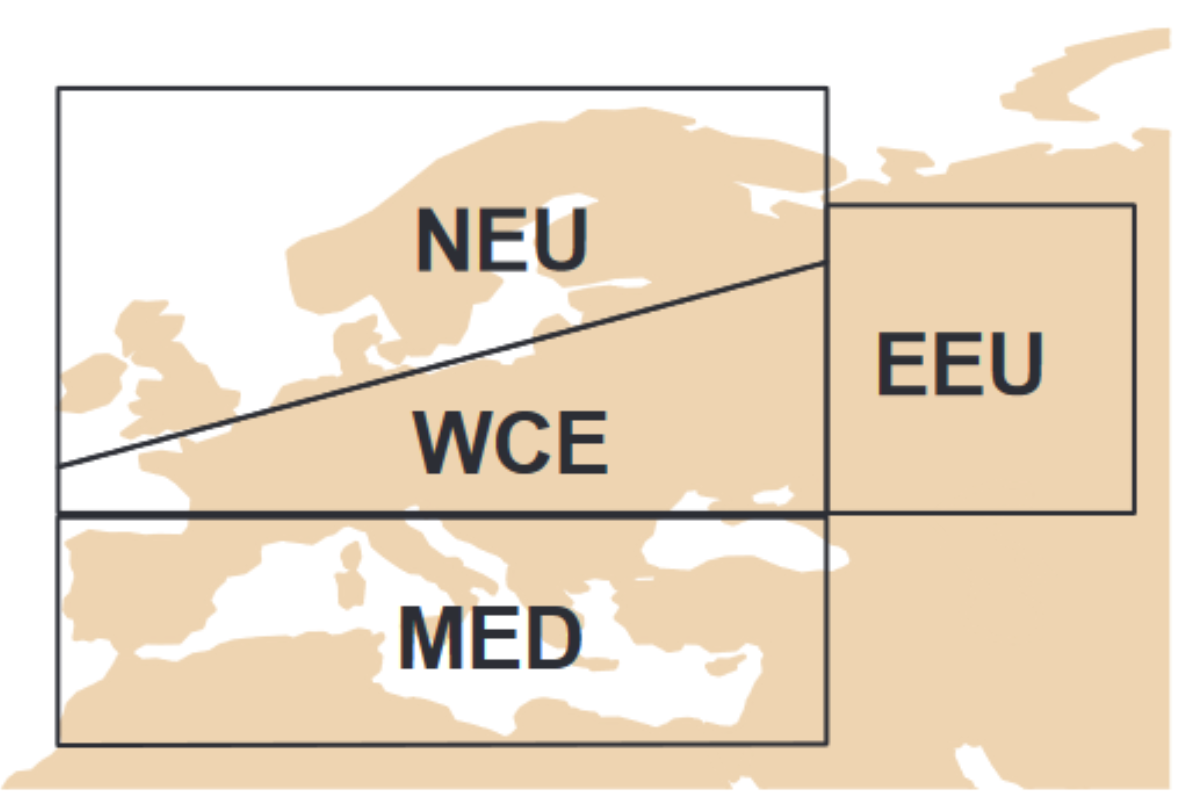
Fig. 19 IPCC climate zones in Europe. Image taken from the IPCC Atlas#
We analyse past climate behaviour by following the next steps:
Select your region
Select the historical observation data set “era5-land”
Select climate impact drivers and season of interest
Click on “Regional Information” for more information
Spot potential trends
Latvian example
As Latvia is situated on the border between NEU and WCE we need to choose which region. Since the European risk assessment considers the Baltic states to be part of NEU we also choose this region. The graphs below are obtained frpm https://atlas.climate.copernicus.eu/atlas. Overall, there has been an upward trend in ERA5 data for precipitation as can be seen from the graph.
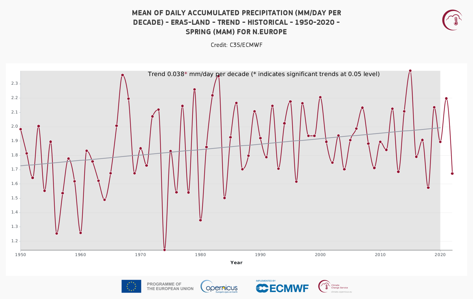
Fig. 20 Precipitation trend in spring for NEU#
In the whole of NEU we find that snow has a slightly increasing trend. The increasing rainfall trend might have contributed to more snow accumulation than temperature increases have reduced snow accumulation.
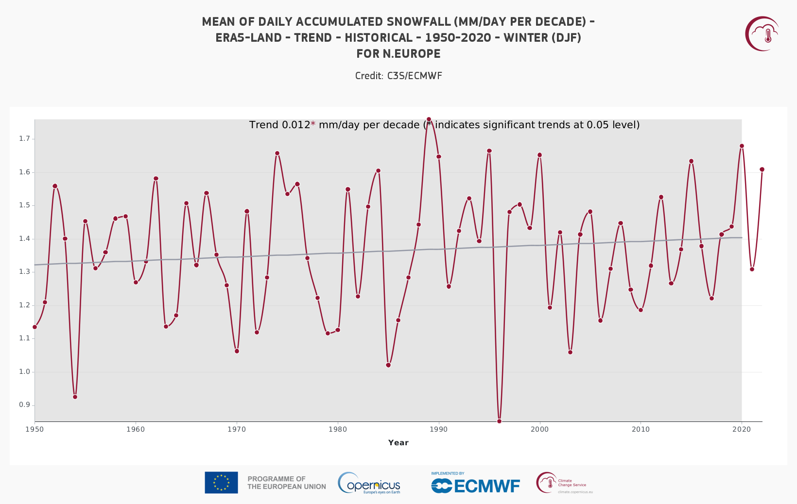
Fig. 21 Snow trend in winter in NEU#
Based on what we know of the climatic impact drivers we would expect that there are slight increases in both snowmelt and saturated soil floods.
3. Collect simulation trends#
For this notebook, we have compiled projections from climate models for each IPCC climate region for various emission scenarios. In the plot below, the horizontal axis indicates the change in the selected climate variable. At the top we have indicated the multi-model means of emisssions scenarios. Underneath, we show the spread of model outcomes from which the multi-model mean was calculated. After you have read through the example feel free to play around with the plot for your region and climate variable of interest.
Latvian example
The figure below is obtained by selecting the change in Total Precipitation for the season Mar-May for the year 2041 for the NEU region. We notice that that the individual model projections span a much larger range of change than the SSP averaged scenarios. Here we see that individual models behave differently towards the same emission scenarios. This can be either due to differences in the way they represent physical processes or because they are subject to randomness of the weather and might have hit a cold snap or dry spell in their simulations.
For precipitation we notice that when emissions increase SSP model mean changes increase. Individual model projections all indicate an increase in spring precipitation, yet the amount is more unclear. When analysing what could happen in the future we see that in each SSP small increases can occur (<5%) while high increases (>15%) only occur under high emission scenarios. When using this information with known flood mechanisms where soils are saturated and extra rain leads to high discharges, we can expect more of these events to occur. An increase of 10% extra precipitation in the spring season is not unlikely across models and can lead to severe changes in discharges.
Snowfall is expected to decrease when emissions, and thus also temperatures increase. Given that Northern Europe historically received roughly 1.3 mm/day of snow in winter the range given is between a 24% reduction to a 7% increase in snowfall. Few models project an increase and this might only be due to randomness of weather. However, 7% extra snowfall in winter snowpack can result into large changes in melt discharges and might be worth investigating as a potential ‘what if’ scenario. A reduction of 24% is also interesting as it greatly limits snow accumulation and therefore the snow melt flood mechanism.
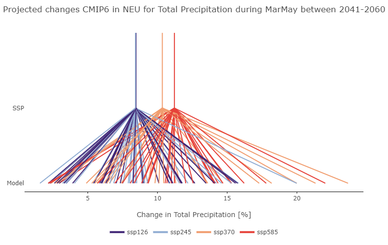
Fig. 22 Plot of uncertainties for climate variable in NEU#
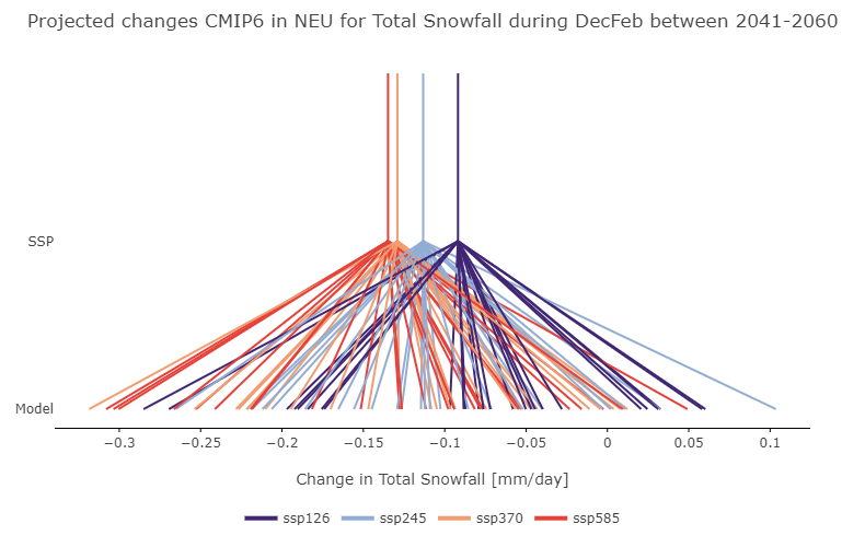
Fig. 23 Plot of uncertainties for climate variable in NEU#
See also
The data visualized above is available from our CLIMATE SCENARIOS GitHub repository.
4. Look into IPCC reports why this occurs#
To get a better sense of why there is such a large range of what could happen in the future we can dive into the IPCC reports to give some clarity. In the reports a scientific background is given to many of the projected changes. To get started we can use ChatClimate. This is an AI tool that is specialised in the IPCC report and guides users towards the chapters and information they need. A good starting point to ask questions is to use the following template.
“What are the expected changes in [region] for [climate impact variable] and why do these changes occur? Also include reasons for differences across climate models.”
if you want to know more or do not understand parts of the answers follow up by using.
“What do you mean by this? [copy text from anwer you want to know more about]”
One can also dive into the IPCC reports and search for explanations. Here are some useful links:
IPCC Climate Change 2021: The Physical Science Basis (for a chapter overview)
Chapter 11: Weather and Climate Extreme Events in a Changing Climate
Chapter 12: Climate Change Information for Regional Impact and for Risk Assessment
Latvian example
Here we dive into the details of why precipitation is expected to increase in Northern Europe and why snowfall is decreasing. Using the information below we have a good basis to dive into the reports if needed or reach out to other experts to tell us more.
Precipitation
When asking ChatClimate: “What are the expected changes in NEU for average precipitation amounts in spring and why do these changes occur? Also include reasons for differences across climate models.” it gives the following answer.
“The expected changes in average precipitation amounts in NEU (North-Eastern Europe) for spring are not explicitly mentioned in the provided information. However, it is reported that in the winter half year, NEU is likely to have increased mean precipitation associated with increased atmospheric moisture and moisture convergence, and intensification in extratropical cyclone activity (Page: 72, Reference: IPCC_AR6_WGI_Atlas). The changes in precipitation are driven by the increase in atmospheric water vapour (about 7% per 1°C of warming near the surface), although this is modulated by various dynamical changes. Changes in average precipitation are also driven by slower processes that constrain future changes over the globe to only 2-3% per 1°C of warming near the surface (Page: 96, Reference: IPCC_AR6_WGI_Chapter11). The differences across climate models are due to pronounced internal variability in this region, particularly NAO (North Atlantic Oscillation) and AMO (Atlantic Multidecadal Oscillation). The spread in climate model projections is still substantial, partly due to these factors (Page: 72, Reference: IPCC_AR6_WGI_Atlas). Additionally, near-term projected changes in precipitation are uncertain mainly because of natural internal variability, model uncertainty, and uncertainty in natural and anthropogenic aerosol forcing (Page: 33, Reference: IPCC_AR6_WGI_Chapter04). However, without more specific information about spring precipitation in NEU, there is not enough info to answer the question fully.”
When asking “What do you mean by this? The differences across climate models are due to pronounced internal variability in this region, particularly NAO (North Atlantic Oscillation) and AMO (Atlantic Multidecadal Oscillation). The spread in climate model projections is still substantial, partly due to these factors (Page: 72, Reference: IPCC_AR6_WGI_Atlas).” We learn more.
“The statement refers to the variability in climate model projections due to internal climate factors, specifically the North Atlantic Oscillation (NAO) and the Atlantic Multidecadal Oscillation (AMO). These are modes of climate variability that can significantly influence regional climates. The NAO, for instance, is the main mode of climate variability over the North Atlantic-European region in all seasons, affecting temperature, precipitation, wind patterns, and even the occurrence of extreme weather events (Page: 4, Reference: IPCC_AR6_WGI_AnnexIV). It can also lead to significant uncertainty in future changes of regional climate, as seen in the CMIP5 RCP8.5 scenario where an increased amplitude and frequency of the NAO during winter is associated with higher precipitation in northern Europe and lower precipitation in southern Europe (Page: 81, Reference: IPCC_AR6_WGI_Chapter08). The AMO, while not explicitly described in the provided information, is another mode of climate variability that can influence climate model projections. The spread in climate model projections refers to the range of possible outcomes predicted by different climate models. This spread is substantial, meaning there is a wide range of possible future climates predicted by these models, partly due to the influence of internal variability factors like the NAO and AMO (Page: 72, Reference: IPCC_AR6_WGI_Atlas). However, it’s also noted that some climate models may have deficiencies that cause the predictable signal associated with the NAO to be weaker than in nature, while others, such as that linked to the SAM, are more consistent with observations (Page: 12, Reference: IPCC_AR6_WGI_Chapter04). This could also contribute to the spread in climate model projections (In-house knowledge).”
Snowfall
When asking ChatClimate: “What are the expected changes in NEU for average snowfall amounts in winter and why do these changes occur? Also include reasons for differences across climate models.”
“The expected changes in average snowfall amounts in winter in North-Eastern Europe (NEU) are likely to decrease due to global warming. This is because regional warming is virtually certain to extend the observed downward trends in snow accumulation, snow water equivalent, and length of the snow cover season in NEU (Page:76, Reference:IPCC_AR6_WGI_Atlas). This is supported by regional and global multi-model and/or single-model ensemble projections including CMIP5, PRUDENCE, ENSEMBLES, and EURO-CORDEX. The changes are attributed to changes in the snowfall fraction of precipitation and to increased snowmelt (Page:76, Reference:IPCC_AR6_WGI_Atlas). The differences across climate models can be due to the different ways they represent physical processes and their interactions. For example, Terzago et al. (2017) showed a large positive bias in the amplitude of the annual snow cycle of EURO-CORDEX 0.11° simulations driven by GCM projections, while reanalysis-driven RCMs showed good agreement with in situ observations (Page:76, Reference:IPCC_AR6_WGI_Atlas). Furthermore, changes in precipitation extremes (including both rainfall and snowfall extremes) can differ drastically from those in average precipitation. The intensification of extreme precipitation is driven by the increase in atmospheric water vapour (about 7% per 1°C of warming near the surface), although this is modulated by various dynamical changes. In contrast, changes in average precipitation are driven not only by moisture increases but also by slower processes that constrain future changes over the globe to only 2-3% per 1°C of warming near the surface (Page:96, Reference:IPCC_AR6_WGI_Chapter11). In summary, the expected changes in NEU for average snowfall amounts in winter are likely to decrease due to global warming, and the differences across climate models can be attributed to the different ways they represent physical processes and their interactions (In-house knowledge).”
5. Advanced steps#
Here we propose some steps that could be taken to gain better insights into the actual impacts of these future trends.
Using climate time series from multiple models in impact analysis
Why this matters: Climate projections come with uncertainty, as no single model can capture the full range of possible futures. By using a set of models that span this uncertainty, you ensure that your projections cover a wide spectrum of possible scenarios. This helps you to account for the unpredictable nature of climate change.
Action: Select a diverse set of climate models that represent different outcomes for the climate impact variables and use these in impact analyses, such as the CLIMAAX risk workflows. This will help you explore the range of potential outcomes, from worst-case to moderate scenarios.
Adjusting historical weather patterns with a stochastic weather generator
Why this matters: Simply applying model projections can be too coarse for the complexity of daily weather variations. By adjusting historical weather patterns based on projected climate signals, you can generate more detailed scenarios of how weather might evolve under future climate conditions. Stochastic Weather Generators also provide a method to increase the length of your time-series enabling extreme value analysis.
Action: Use a stochastic weather generator to blend the climate signals from the models with observed historical weather data. This process can mimic how variables like temperature and precipitation might shift, while preserving local conditions.
Use these projections in combination with socioeconomic changes
Why it matters: The severity and impact of climate change depend not just on the physical climate but also on how societies evolve. Integrating climate projections with different socioeconomic scenarios allows for more holistic scenarios, reflecting changes in population, technology, and governance that either increase or decrease vulnerability.
Action: Combine your climate model outputs with scenarios of regional socioeconomic development. For example, increased precipitation combined with rapid urban growth may result in higher risks than the same climate future with strong policy intervention and innovation. Use such combinations to explore how risks might change based on both climate and socioeconomic dynamics.
