Working with vulnerability curves

The following aims to guide enhanced damage estimations in the region. The damage estimation in a region for a flood or windstorm is created by finding how much can possibly be damaged multiplied by a percentage of what is actually damaged based on the severity of the hazard. A guide for the local estimation of maximum damages per square meter is given, together with a description of how standard vulnerability curves can be adapted to fit the local or regional situation. In this method, standard damage estimations and damage curves from literature are adjusted to the local context using local knowledge. The two final products are a table with custom maximum damage per land use and a set of damage curves for the various land uses in the region. shows an overview of how to refine general data to the local context.

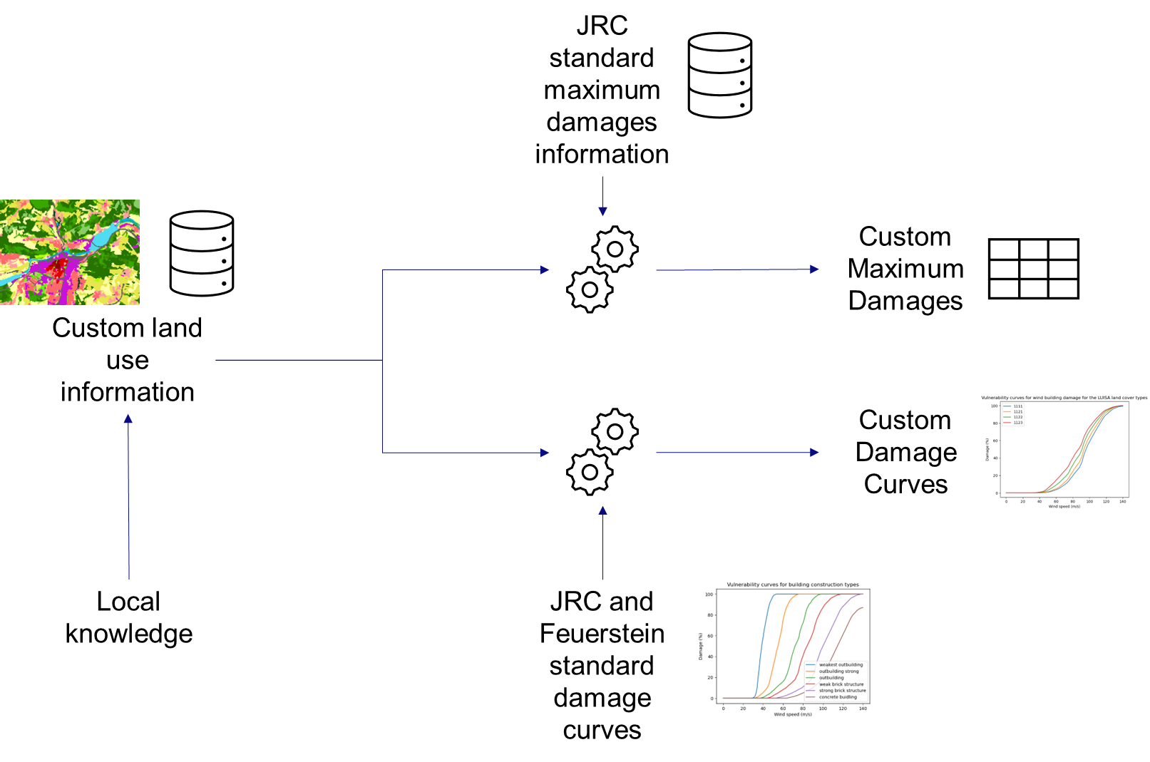
Fig. 33 In this method, standard damage estimations and damage curves from literature are adjusted to the local context using local knowledge. The two final products are a table with custom maximum damage per land use and a set of damage curves for the various land uses in the region.

1.    Maximum damage estimations

The first step to be taken is to find estimations of the maximum damage per square meter of the assets that represent in the region. This can then be used to find actual damages by combining maximum damages with the actual fraction of loss based on the severity of a windstorm or flood event.

Table 1: Description of flood damage classes as defined by Huizinga et al. (2017)

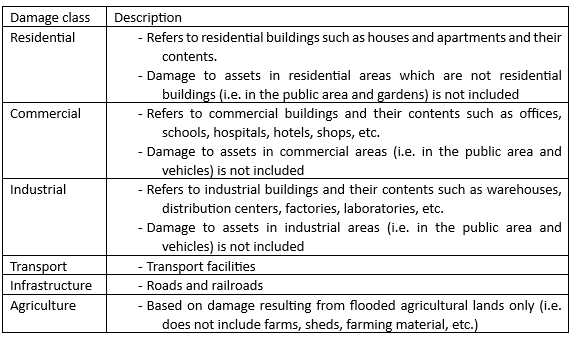
Max damage determination of building footprints Commercial, Residential, Industrial

The maximum damage that can occur to a building is a combination of construction costs and the value of the content inside a building. When a flood occurs, the building is damaged but also the furniture, machines, or store inventory is affected. First, the construction cost is determined. When building costs are known in the region, this value can be filled in directly. Otherwise, the following relation found by Huizinga et al. (2017) can be used to calculate the construction cost for buildings per square meter. Huizinga et al. assume different building costs per type of building. The provided relations are for residential, commercial, and industrial buildings.

(1)\[construction\ cost/m² = a * GDPper\ capita_{year\ x}^b\]

Table 2: Empirically found values for building use classes (Huizinga et al., 2017)

(2)\[a_{landuse}=\ R_{res}\ast\ a_{res}+\ R_{com}\ast\ a_{com}+\ R_{ind}\ast\ a_{ind}\]

(3)\[b_{landuse}=\ R_{res}\ast\ b_{res}+\ R_{com}\ast\ b_{com}+\ R_{ind}\ast\ b_{ind}ated assets \]

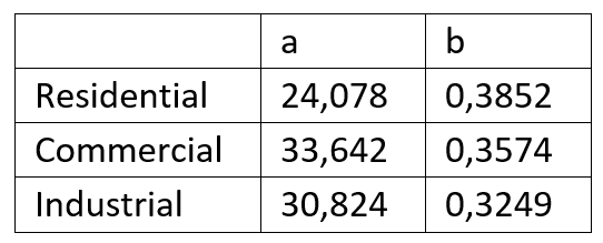
where:

\(a_{landuse}\) = the new a variable for the land use raster
\(b_{landuse}\) = the new b variable for the land use raster

\(R_{res}\) = ratio of residential assets in the specific landuse cell
\(a_{res}\) = the a variable for the residential-related assets
\(b_{res}\) = the b variable for the residential-related assets

\(R_{com}\) = ratio of commercial assets in the specific landuse cell
\(a_{com}\) = the a variable for commercial-related assets
\(b_{com}\) = the b variable for for commercial-related assets

\(R_{ind}\) = ratio of industrial assets in the specific landuse cell
\(a_{ind}\) = the a variable for industrial-related assets
\(b_{ind}\) = the b variable for industrial-related assets

(4)\[Max\ damage\ structure/m² = construction\ cost/m² * depreciated\ value * (1- undamageable\ percentage) * materials\ used\ factor\]

Table 3: Indicatory values for the ‘materials used factor’ (Huizinga et al., 2017)

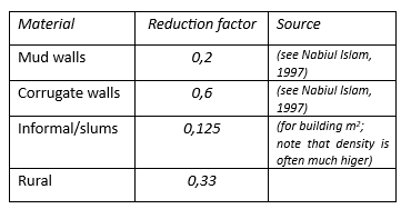
Table 4: Indicatory values for the undamageable percentage in equation X (Huizinga et al., 2017)

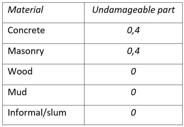
When the maximum damage of the structure is known, the content damage can be estimated by multiplying the structure damage with the content importance factor. It estimates how much the content is worth based on how valuable the building is.

Table 5: Indicatory values for the importance of content factor (Huizinga et al., 2017)

(5)\[f_{content}=\ R_{res}\ast\ f_{res}+\ R_{com}\ast\ f_{com}+\ R_{ind}\ast\ f_{ind}\]

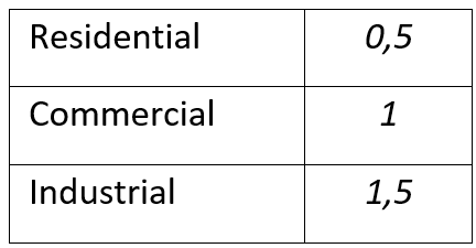
Where:

\(f_{content}\) = the new conversion factor for the importance of the content in the land use raster

\(R_{res}\) = ratio of residential assets in the specific landuse cell
\(f_{res}\) = the factor importance of content for residential-related assets

\(R_{com}\) = ratio of commercial assets in the specific landuse cell
\(f_{com}\) = the factor importance of content for commercial-related assets

\(R_{ind}\) = ratio of industrial assets in the specific landuse cell
\(f_{com}\) = the factor importance of content for industrial-related assets

The total damage per square meter can then be defined by adding the maximum content and structural damage together.

(6)\[Total\ damage/m² = Max\ damage\ structure/m² + Max\ damage\ content/m²\]

Max damage determination for land use data Commercial, Residential, Industrial

When working with land use data that has a raster format a single cell is not necessarily filled completely by building footprints. That is why a density factor is needed to go from a fully build up land use cell to one which contains some ‘empty space’ between buildings.

(7)\[Total\ damage/m²_{landuse} = Total\ damage/m² * percentage\ of\ area\ covered\ by\ building\ footprint\]

Max damage determination for Agriculture

Per land use type of agriculture, the value added can be changed to get some differentiation between the types of farming that is being done.

(8)\[Value\ added/m² = \frac{Value\ added/hectare}{10\ 000}\]

Max damage determination for Infrastructure, Transport

(9)\[Damage/m² = \frac{Maximum\ damage_{average} * GDP_{country}}{GDP_{average}}\]

2. Vulnerability curves

Next to the value of the assets it is also important to find how vulnerable an asset is to a certain hazard. One way to do this is by identifying vulnerability curves. These curves relate a hazard intensity to a fraction of the maximum damages that occurs under this hazard intensity. In the next section, vulnerability curves for floods and windstorms will be elaborated.

Flood

For flood damages, Huizinga et al. (2017) quantified the depth-damage curves across the world, see Figure 1. These depth-damage curves relate the water depth during a flood event to a fraction of the building that is damaged. This fraction is multiplied by the found maximum damage of a certain asset in Section 1. The authors have six classes of asests: residential, commercial, industrial, agriculture, transport, and infrastructure – roads

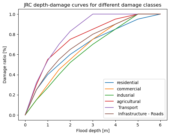
Fig. 34 Flood vulnerability curves as found by Huizinga et al. (2017) and used by the JRC

Raster-based land use data may not contain information on the distribution of damage classes within the land use class. This will then need to be estimated by the stakeholder per land-use class. These proportions can then be used to create a new depth-damage curve that considers the proportions of buildings in the land use cell. See the formula below.

(10)\[c_{new}\left(m\right)=\ R_{c1}\ast\ c_1\left(m\right)+\ \left[\ldots\right]+\ R_{cn}\ast\ c_n\left(m\right)\]

Where:

\(c_{new}\ (m)\) = the new curve for the land use class as a function of inundation depth
\(m\) = inundation depth
\(R_{cn}\) = ratio of class type in the specific landuse cell that should have curve n
\(c_n\ (m)\) = curve for asset type n as a function of inundation depth

Wind

For wind, the vulnerability curves are based on the construction type of a building. Some structures are more resilient than others. For example, wooden sheds are easier to be damaged by wind than concrete buildings. Using the selection of Feurstein et al. (2011) six vulnerability curves can be differentiated.

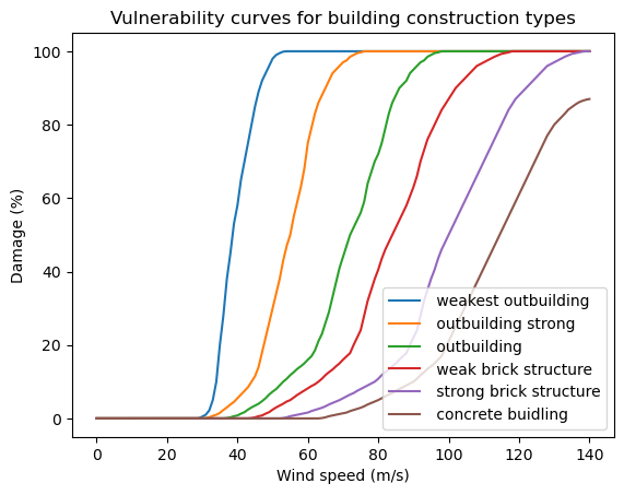
Fig. 35 Vulnerability curves as found by Feuerstein et al. (2011)

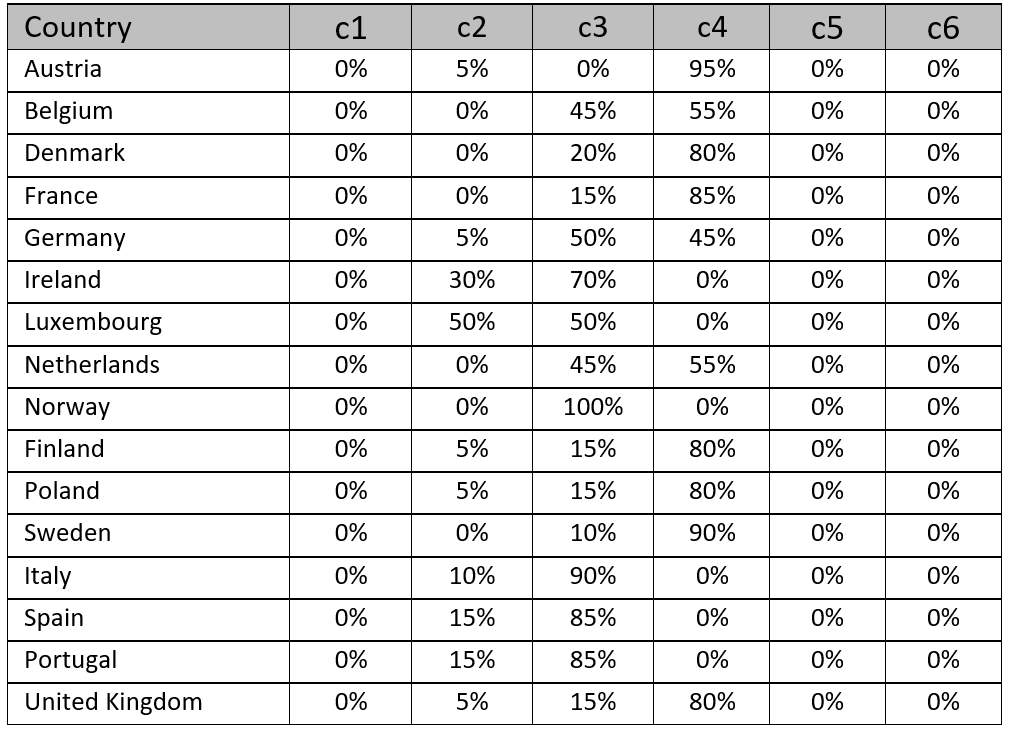
Land use data contains no information on specific building types and this needs to be estimated by the stakeholder per land use class. However, as a first estimation, the PAGER database is used by (Koks & Haer., 2020) and a table is given here. to identify the proportion of building types per land use. These proportions can then be used to create a new curve that considers the proportions of buildings in the land use cell.

(11)\[c_{new}\left(w\right)=\ R_{c1}\ast\ c_1\left(w\right)+\ \left[\ldots\right]+\ R_{cn}\ast\ c_n\left(w\right)\]

Where:

\(c_{new}\ (w)\) = the new curve for the land use class as a function of windspeed
\(w\) = 3-second windgust in \(m/s\)
\(R_{cn}\) = ratio of class type in the specific landuse cell that should have curve n
\(c_n\ (w)\) = curve for building type n as a function of windspeed

Table 5 Table with curve ratios identified by per country that results in damage values similar to losses from other models. As found by (Koks & Haer., 2020)

3. References

Huizinga, J., De Moel, H. and Szewczyk, W., Global flood depth-damage functions: Methodology and the database with guidelines, EUR 28552 EN, Publications Office of the European Union, Luxembourg, 2017, ISBN 978-92-79-67781-6, doi:10.2760/16510, JRC105688.

Koks, E. E., & Haer, T. (2020). A high-resolution wind damage model for Europe. Scientific reports, 10(1), 6866. doi: 10.1038/s41598-020-63580-w